Ever since my grandparents first pulled out the “outer space” placemats I’ve had a healthy interest in the stars. After attending a couple of NETS conferences, hosted by the American Nuclear Society, I seized an opportunity to make my own contribution to the space industry by modeling a Nuclear Thermal Propulsion engine in Flownex.
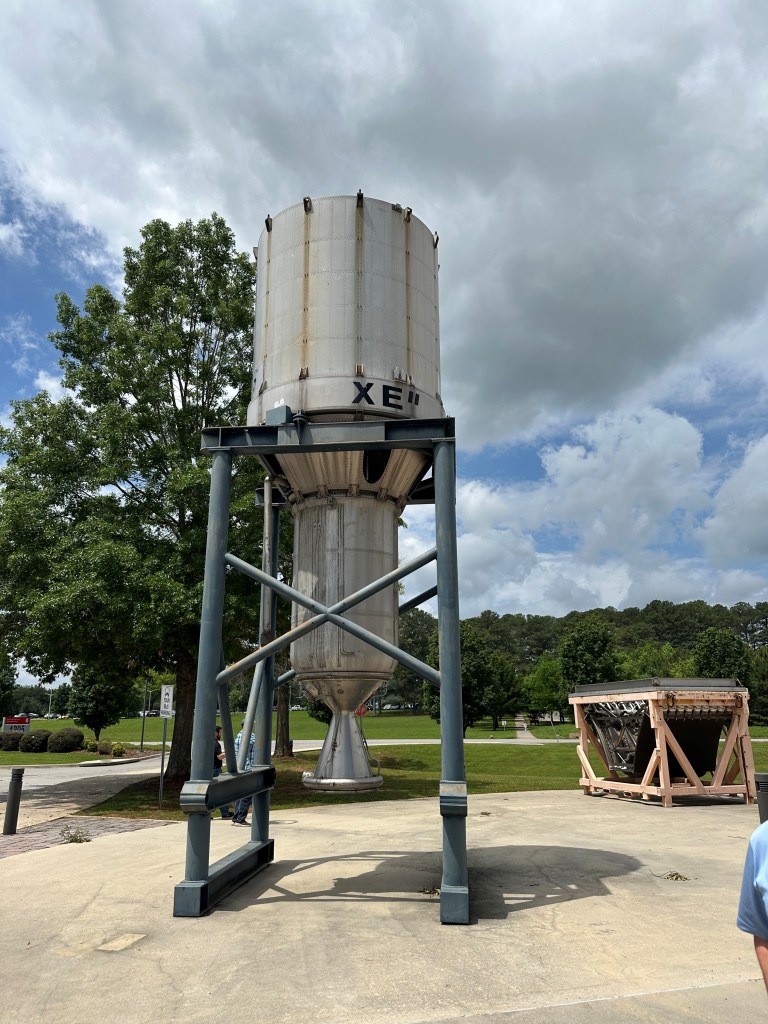
XE Prime at
The reason for this effort is two-fold. First, I just wanted to see if it could be done. Second, in my experience at these conferences, lots of really smart scientists and engineers are developing outstanding novel technologies and designs, but spend a large effort solving the thermal-hydraulics of their systems manually or through custom scripted routines. I suspect it would benefit the entire industry if we can enable the scientists to focus on the science by qualifying existing tools (like Flownex) on difficult applications, like nuclear thermal propulsion.
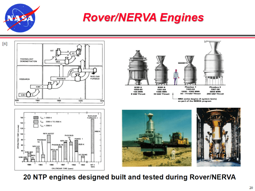
I cleared this effort with my boss and our marketing department, now I needed to find an example. Nuclear thermal propulsion has existed as a theoretical technology for space transport since the 1940s. In ~1955 Los Alamos began development work on NTP engines with Project Rover. Then, in 1960, NASA, in collaboration with the Atomic Energy Commission opened the Space Nuclear Propulsion Office. This brings us to NERVA – Nuclear Engine for Rocket Vehicle Application, which was the child of these organizations marriage and a continuation of the Project Rover effort.
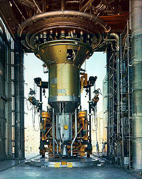
As part of the NERVA project several conceptual NTP engines were designed, built, and even test fired.
I began parsing through old reports, presentations, and test data. There was a ton of material to sift through. Much of it poorly xeroxed. One of the reports I was interested in was only available as a microfiche scan at a university library. The good news is that filtering through all of the available reports and data, there was a clear choice for an engine which had flow diagrams, geometry, some reactor details, and most important, test results for a range of operating conditions! The Xe-Prime.
See how Flownex, ADT TurboDESIGN, and Ansys can be used to expedite and optimize turbopump design for propulsion systems in this joint webinar presented by PADT and ADT.
Hi Folks! Another short and simple tech tip this week; How to set up an external shared database in Flownex. When working as part of a team it makes sense to share resources. Once one person builds a custom component or defines a complex fluid we want to share that with everyone in our organization. Today I will show you how to create and maintain a shared database. For todays example we are working in Flownex version 8.12.7.4334
Creating the Database
Start by opening up Flownex – it can be a new project or any existing project. On the right side of the GUI we’ll want to navigate to the Components pane. At the top of the pane you’ll see a variety of buttons. Depending on your installation the buttons you see may be different than the ones in the visual below. To create a new database we’ll want to click the Create Database icon.
Then we’ll want to navigate to a shared network location and pick an appropriate folder that will be accessible to others in our organization. I would encourage keeping the directory name as short as possible (I.E. a top level location) so that there is no concern for a deep database hitting windows character limit.
Once we have chosen a location and clicked OK we will see our shared database in both the Components pane and in the Charts and Lookup Tables pane. We’ll need to right-click on the newly created shared database and create a New Library in which we will place our shared components. Creating multiple libraries can be useful when grouping similar components or to discretize between different groups in the organization which are using Flownex.
Adding components to an External Database
To add custom components to our external database we simply drag and drop them from our project database. If you want to learn how to create a custom compound component please reference our previous blog post on this topic here. Choosing “Copy” will create a copy of the component in the shared database, choosing “Move” will move the component to the shared database and any references to that component in the project will now reference the component from the external database.
Adding a fluid to an External Database
To add a custom fluid to our external database the process is very similar to the procedure for the custom compound component. The only difference is that we want to do this drag and drop action within the Charts and Lookup Tables pane instead of the Components pane. If you need a refresher on creating or importing custom fluids here is a blog post on that topic!
Connecting to an External Database
Once a user has created a shared database it is now possible for other users to connect to that database. the process of connecting to an external database is quite simple. On the Components pane we will again look at the buttons near the top. We will want to click the Connect Database icon and then navigate to the shared location of the external database. Once there we will find the database configuration file, .dbcfg. We should select this file and click OK. You are now connected to the shared database!
Bonus Tips!
To lock an external database to avoid unintentional editing you can right-click on the database in Flownex and select “Lock Database”.
If you need to migrate the database to another location on your server you can copy the entirety of the folder and move it. Users will simply need to follow the same procedure of connecting to an external database the next time they open Flownex.
Special Note: If sending a network to someone external to your organization it is important to note that components or references from external databases will not be included by default. These components or charts will need to be copied to the project database and then the shared database will need to be disconnected before archiving the project for transfer. A second option would be to share the database itself.
Occasionally glossed over, adding custom fluids is a fairly standard operation in Flownex that we don’t think about until it’s necessary. There are a couple of ways to do this which we’ll go over in today’s post. I am working in Flownex 8.12.7.4334.
Creating a mixed fluid
To create a mixed fluid we first need to create a folder for this fluid in our project database. This can be done in the charts and lookup tables pane by right clicking on “mixed fluids” and selecting “add category”. We can create our new fluid by right-clicking on the new folder and selecting “Add a new mixed fluid”. Note we can right-click and rename both the fluid itself and the containing folder.
To define our new mixed fluid we double-click on the new mixed fluid to open the editor. Here we can add the components of our mixed fluids.
Creating a new fluid from scratch
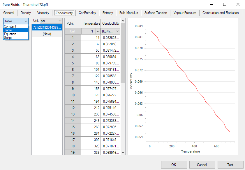
To create a fluid from scratch we repeat the same process of creating a folder and creating a new fluid as above with the exception being that we’d complete these steps under the “Pure Fluids” category. Once this is done we’ll need to double-click or right-click > edit our from scratch fluid and enter in the fluid properties. Note for many properties we can define the relationship with pressure and temperature as constant (non-dependent), table, equation, or script.
Importing a fluid
To import a fluid we will follow the same steps of creating the folder under pure fluids. Now instead of right-clicking and adding new we will right-click and select “import”. Then we simply navigate to our desired fluid file and click “Ok”.
Bonus Tips!
In the window where you define your fluid you’ll notice the “Test” button. This feature can be utilized to test created fluids to confirm properties against known properties for given pressures and temperatures.
We can also copy and paste fluids from the master database into the project database to give us a good starting point for creating similar fluids (or extending properties to higher/lower temps/pressures).
The result layers in Flownex have evolved quite a bit over the last few iterations of the code. Although we might typically associate color-gradient results more with 3D CFD, it does have a place in 1D system modeling. Taking advantage of results layers in Flownex can give a very quick understanding of what is going on with our system, and, with a little customization, can be incredibly powerful as an addition to our design and analysis toolbelt. In this post I am using Flownex version 8.12.7.4334.
How to create a result layer
To create a custom result layer we must navigate to the results ribbon and select result layer setup.
First we want to right-click in the Result Layers window and add a new result layer.
There are two options to add the schema for our result layer. The first is to right-click on the Selected Result Layer Schemas and add either a specific or generic schema. The second, and my PREFERRED, method is to simply drag and drop results from components on the canvas into this window:
Note that I want to multi-select any component types which will be included in this result layer. This could be any flow components which share a common result such as “quality”. I also convert to generic because I want the result layer to apply to all pipes, not just the pipe I initially drag and drop the property from.
Defining the custom result layer
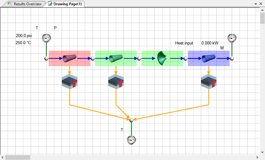
In this example I have a two-phase water network with a cold external temperature. I want to create a result layer to quickly see if the water is in the gas phase, liquid phase, or somewhere in-between. The problem I have been tasked with solving is ensuring that the water never condenses. I will need to determine where we may need to add additional heat flux to the network.
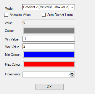
We can use the Quality result property to determine the phase of our fluid. Quality < 0 indicates fully liquid, quality between 0 and 1 indicates liquid/gas mixture, greater than 1 indicates fully vapor.
To make this work as intended I can set up a gradient with three increments going from -1 to 2. The idea being the lowest increment would encompass -1 to 0, middle increment would be 0 to 1, and the top increment would be 1 to 2. For the gradient mode I made sure to pick <-[MinValue, MaxValue]-> so that the max and min increments would extend past the specified range.
As we apply this to our network we can easily see that we do, in fact, have a phase change from gas at the inlet, to mixture in the second two component, to fully liquid near the outlet.
I may decide to add a heater to our outlet pipe and perhaps a thicker insulative layer to all three to attempt to keep the water in gas phase throughout the system.
Bonus Tip!
Result layers can also be super handy when troubleshooting to quickly identify large pressure differentials, choking points, or other outlying fluid properties.
Compound components make it easy and efficient to reuse the same collection of components over and over throughout your models. In this post I’ll be going over the basics of making a user-friendly and aesthetically pleasing compound component. In this example I am working in Flownex Version 8.12.7.4334
How to create a compound component
To create a compound component we must first create a local library in the project database. This can be done by right-clicking on the project database in the components pane and select “New Library”.
We can name our new library and choose a picture if desired:
To create our compound component we just need to right-click on the new library and select “New Compound Item”
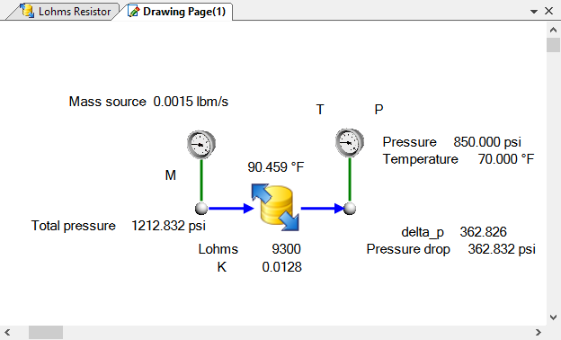
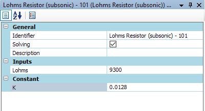
To build our compound component we’ll use the “edit” function on the compound component. In this example I am building a Lohm resistor component. It’s a good idea to test my component on a separate page to make sure scripts interact as expected and validate results against some given test cases.
Let’s make it functional!
To define the inputs and results we’d like to expose to the user we right-click on the new compound component in the library and select “component setup”.
To add inputs and results we need to navigate to the Compound Setup ribbon and then simply drag and drop inputs and results into the Selected Properties window. Note that we can even grab whole categories of inputs or results to save time!
Now those inputs and results will appear to the user when they add this compound component to their canvas!
Let’s make it pretty!
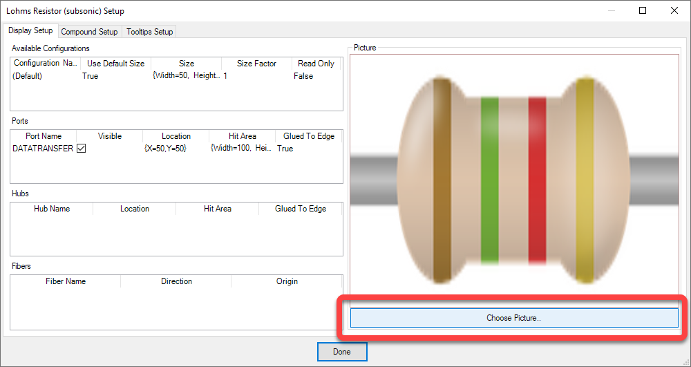
To make our component more aesthetically appealing let’s replace the boring default icon with one more representative of our Lohm Resistor. To do this we right-click on our compound component again and this time stay in the “Display Setup” tab. We can click the “Choose Picture” button to upload our own icon. To refresh on the image selector check out the blog post on adding a background image.
To correct the aspect ratio so that it shows up looking less squished on our canvas we want to change the settings back in the Compound Setup tab. I’ll change it to 133×34 so that it appears similar in scale to the standard flow components but correct in the aspect ratio.
Now when we place our compound component onto our canvas it should look great!
Bonus Tips!
In the compound component setup there is a third ribbon called “Tooltips Setup”. This is where we can define what properties show up when we hover our mouse over the component.
Don’t forget we can save compound components in a “database” on a server so that they can be accessed by every Flownex user in your organization.
Building on last week’s global parameters example I’d like to show some tricks within the input sheet environment. These are really more so excel tricks – but the methodology within Flownex is slightly different. In this example I am working in Flownex Version 8.12.7.4334
Refresher on using Input Sheets
To create a new Input Sheet we will navigate to the project tab, then select “Excel Reports/Pages”, right-click on the Input Sheets folder, and select “New Input Sheet”
To add inputs to the sheet it’s as simple as dragging and dropping the inputs from the component into the desired cell in the Input Sheet.
Formatting our Input Sheet
I like to use color, shading, and border to specify which cells contain inputs so that if I pass the project off to a client or colleague it is immediately clear what variables they should be editing and which cells they shouldn’t change.
To modify the formatting we need to enter “workbook designer”. This is done by right-clicking on the input sheet and selecting “workbook designer”
All of the standard Excel-type formatting is available here, including adding graphs, images, etc. Typical operations are found in the format menu on the top ribbon.
Drop Downs
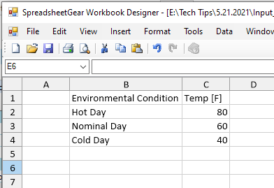
A more advanced Excel operation I like to integrate into these types of input sheets is a drop-down where multiple inputs may be tied to a given condition. In the example below I set up a scenario for given ambient temperature for cold day, hot day, and nominal day.
In the workbook designer we will click “insert” > “worksheet” and build our list of environmental conditions. On the right we will set the associated temperatures.
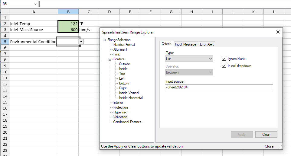
Back on Sheet1 we will need to set up the data validation cell reference to this table. Select the cell where we want to add the dropdown and go to data > validation. We will choose list, and reference cells B2:B4 of Sheet2.
We will need to use VLOOKUP to associate the temp to another cell based on this dropdown. Where this becomes valuable is when we have many input variables tied to each of the dropdown selections.
In this example, since we’ve put the applicable temps a single column to the right the syntax for VLOOKUP will be “=VLOOKUP(B5,Sheet2!B2:C4,2,FALSE)”. After this is added it should behave as follows:
As I mentioned before, this trick becomes very powerful when you have many different environmental or operational inputs tied to a single “scenario” that you want to model in an individual run rather than in a parameter study.
Bonus Tip!
All of these tricks can be applied to any of the excel-type sheets within Flownex. Remember to be careful with parameter tables as the inputs and results are tied to the columns instead of individual cells.
As we build more and more networks it quickly becomes tedious to enter in the same inputs many times. There are a couple methods of using global parameters to save us lots of time and clicks. In this example I am working in Flownex Version 8.12.7.4334
Refresher on Global Parameters
Global parameters are just what they sound like. Parameters defined globally for the project. These could be any type of component input; diameter, length, temp, pressure, etc.
The global parameters can be found in a couple of locations. Under the configuration ribbon we can open the global parameters in a floating window which gives us a friendly interface for creating or modifying these parameters. To create a global parameter one may simply right-click in the GlobalParameters window and select Add (hint: there’s a better way!).
Conventional method to add Global Parameter
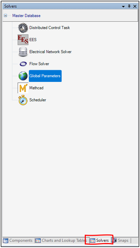
Global parameters can also be accessed in via the solver tab in a similar way to typical inputs (this is important later on).
Access via Solver Tab
The Quick way to add Global Parameters
We don’t really want to have to navigate to that configuration ribbon, right-click a bunch, choose names and assign units do we? Good news! There is a much faster way to add a global parameter. We can add a global parameter with minimal work by simply typing a dollar sign “$” prefacing the name of the tag in any of our component input fields! Remember to hit enter after typing the identifier.
Global Parameter Shortcut
Once a global parameter has been defined we can tie more inputs to the existing parameter by typing the dollar sign “$” and choosing the correct parameter from a drop down:
Multi-Assign Global Parameters
As you can see, this can be quite a time saver when building a network! The next trick utilizing global parameters will have to do with using them for actual analysis.
Using Global Parameters as Manipulatable Inputs
The default/slow way to change a global parameter would be to go to the configuration ribbon > global parameters, and manually change the value in the floating window. No thanks. This is not automated at all and requires many clicks.
The better way to utilize the global parameter as an input would be to tie the global parameter to an input sheet, parameter table (for a parametric study), or even a human machine interface component (HMI).
Global Parameters in Input Sheet
For a design variable that an analyst or engineer may change which would then remain constant (such as pipe diameter) the input sheet comes in very handy. To reference a global parameter in the input sheet recall the second method to access the global parameters and then simply drag and drop onto the input sheet:
Global Parameter in Input Sheet
Global Parameters in Parameter Table
If you are trying to run a parametric study where you are varying something like ambient temperature, it makes sense to use a global parameter as you may have many boundary conditions defined by a single global parameter. Similar to the input sheet this can be tied to a global parameter by a simple drag and drop operation:
Global Parameter as variable in Parameter Table
Global Parameter in a Human Machine Interface
By now I expect you are catching on. The trick to defining a global parameter externally is to use the second method; solver tab > global parameters, and then drag and drop to your desired connection. In the HMI instance I’ve tied inlet mass flow to a Track Bar so that a user can dynamically change the flow rate during the solve:
Global Parameter tied to HMIGlobal Parameters and HMI components
Global Parameters are efficient and POWERFUL
We can use global parameters during network construction using the “$” shortcut to build our networks much more quickly and keep identical inputs the same. We can tie these global parameters to other tools to keep our user inputs all in one place, reducing clicks, and reducing the chance of forgetting to update an input.
Bonus Tips!
Global Parameters can also be used in Designer so that you can keep your independent to dependent variable count the same (EX: Adjusting ALL pipe diameters to target a single exit flowrate)
Global Parameters can be adjusted via transient actions (EX: Adjusting ambient temperature to model the changing temperature over the course of 24 hours).
I’m going to attempt to write a recurring blog post on Fridays with tips and tricks in Flownex that I have discovered over the years. This post will be the first of many! If you enjoy please subscribe.
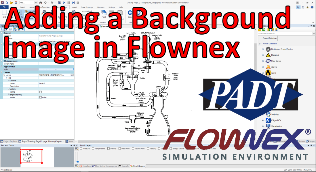
Flownex Tech Tip #1
In this post I will go over what is usually the first step in any network I build. Adding a background image not only helps me lay out my network but also helps colleagues and clients understand networks at a very quick glance. In this example I am using Flownex version 8.12.7.4334
Choosing an Appropriate Image
The first thing we want to do is to make sure that the image size is such that it’s reasonable in size both resolution-wise (so it doesn’t appear pixelated), and right-size so that components don’t appear too small when placed on top. I recommend something in the multi-thousands of pixels both in width an height. 3000 pixels at a minimum. I usually shoot for around 10,000 wide by 5,000 high if the background image will be landscape. For very complex, large networks, it may make sense to go much larger.
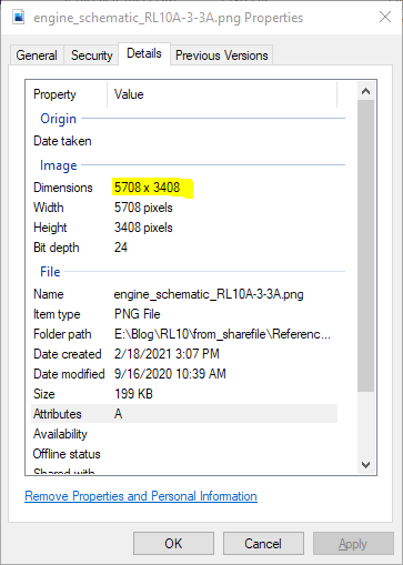
Once we’ve found an appropriate image we will want to make a note of the exact size. This can be found by right-clicking on the image file, selecting properties, and navigating to the details tab.
Confirming Image Resolution
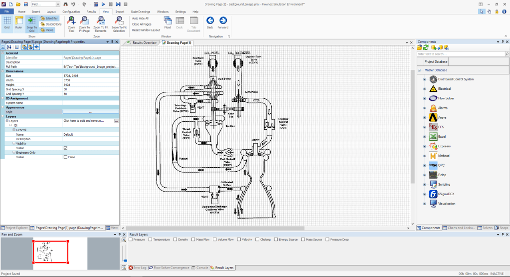
Resizing Flownex Canvas
The canvas in Flownex can be resized to match this resolution by right-clicking on the canvas, selecting edit page, and populating the correct inputs:
Editing Canvas Inputs
Applying Background Image
The background image can be applied by clicking the radio button next to Style in the Appearance subcategory. Here we will change the Fill Style type to Image, then click the Select Image button:
Styles Editor
The images saved locally to this project will appear here. To add an image we simply click Add Image, navigate to the image of our choice, and click open. Now that it is available as an option we select the image in the Image Selector Gallery and click OK.
Image Selector Gallery
We can press OK in the Styles Editor to confirm our changes and we should now see our added image as the new background!
Drawing Canvas with Background Image
Bonus Tips!
Adjusting the Fill Style opacity can fade out the background image so that it doesn’t overwhelm the Flownex components placed on top.
Turning off the grid under the View ribbon can make the canvas a bit more aesthetically pleasing and makes it easier to read text on the background image.