The smell of fireworks and freedom is in the air! This year, my contribution to the family’s Independence day festivities is a smoked brisket. Unfortunately, I have learned from experience that cooking at elevation (~7000ft) is not the same as it is in the valley (~1000ft). To avoid potential embarrassment it only makes sense to run a few simulations before lighting the smoker.
Why?
Smoking a brisket can be tricky, some would say it’s more of an art than a science but at PADT science is our art so we’re going to lean into the science hard. It can take anywhere from 6 to 24 hours to smoke a brisket depending on a variety of factors. Let’s identify what those factors are;
Weight of the Brisket
The Moisture Content of the Brisket
Air Flow
Ambient Air Conditions
The influence of the weight (or mass) of the meat is the main influencer of overall smoke time. The bigger our cut, the more time it’s going to take to smoke. Air flow is going to affect the oxygen available for combustion, effecting the energy available for cooking the brisket, as well as having an effect on heat transfer from the hot air to the brisket. The ambient air conditions will have an effect on energy requirements, heat transfer, and the boiling point of water.
Brisket Stall
The moisture content is going to be our trickiest variable to monitor. We want our brisket to come out of the smoker juicy but as we heat the beef we will evaporate some of the water. This is where the term brisket stall comes from. We eggheads may be more familiar with the scientific description evaporative or adiabatic cooling.
At a certain temperature and pressure water boils and becomes a vapor. This phase transition takes energy, which we are providing by combusting wood chips or pellets, in my case, bourbon barrel oak. Unfortunately, when we hit this critical point we may see all of the energy going to converting water to vapor. Losing too much moisture to vaporization can ruin our brisket. We might increase combustion to add more heat and end up overcooking the meat. We could wait it out and end up drying out the brisket. Worst case scenario is a combination of both!
To avoid this issue many backyard barbecuers recommend the Texas crutch. The brisket can be wrapped in foil or butcher paper. This helps us overcome the stall point by putting a physical barrier in place to reduce the ability for the water vapor to escape the meat.
The Birth of a Brisket Digital Twin
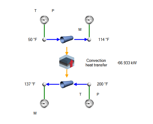
Okay, so not exactly a digital twin. Maybe next time I will incorporate sensor data into the model via OPC server but for now we’re keeping everything digital. I’m using a thermal-fluid modeling tool called Flownex to create a 1D simulation of our brisket and smoker.
The brisket is being modeled using a compound component. I’ve iterated a few times on how exactly I wanted to model it. For the first iteration I kept it simple and used a solid node with an assigned mass and custom solid material characteristics for beef across a temperature range [Baghe-Kandan et, al].
Unfortunately, although our beef’s thermal characteristics (conductivity and thermal capacitance), is temperature dependent, we do not observe the characteristic stall associated with the adiabatic cooling near the boiling point of water. This is due to not modeling any water evaporating, duh.
Beef Brisket V2 was also a failure. I tried to model the solid portion of the brisket separate from the water with heat transfer between the two. It kind of worked, but was needlessly complex, and I didn’t see any effect of a change in elevation on the cooking behavior.
For Beef Brisket V3 I went back to basics. Forget about the smoker, lets just model the solid and liquid that makes up the meat with an applied heat flux and see if we see the stall happen in transient.
The beta testing for V3 was successful! As seen in the above recording, we can see a huge drop in temperature of our solid as soon as our temperature reaches the boiling point of water. We also can see the difference between a sea level analysis and one representing a system operating at 7000 feet above sea level. For the final version of our brisket model I swapped out the two-phase tank with a open container component (to let our water evaporate to atmosphere), and added script to do some basic calculations.
Transient Simulation and Conclusions
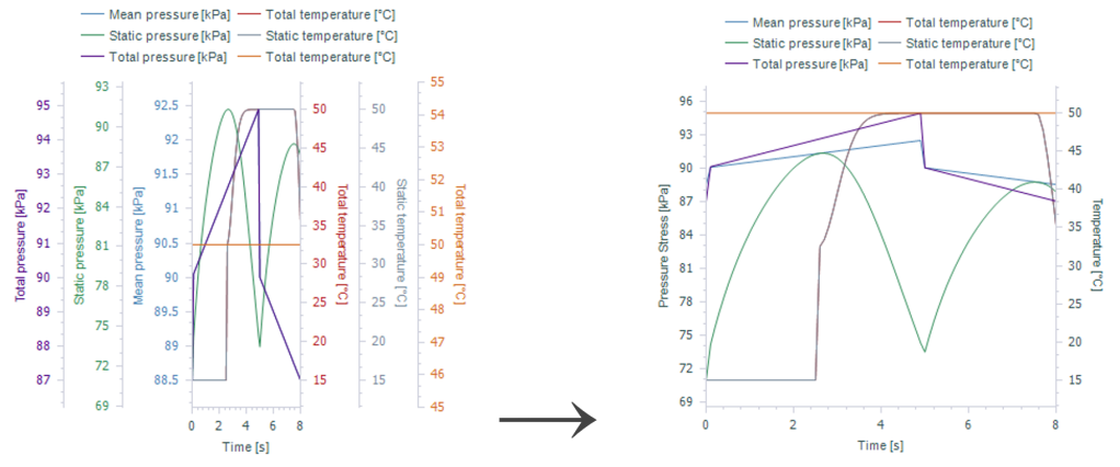
Let’s run the transient simulation in parallel for a smoker at sea level and a smoker at 7000 feet elevation and see what happens!
As we can see in the above transient analysis both briskets experience “stall” once the water begins to evaporate. The brisket at elevation hits its stall at around 199°F, at around the 6 hour mark, the brisket at sea level stalls at 212°F near the 8 hour mark. What this means is that if we are fighting an impossible battle if we try to hit the typically recommended 205°F pull temperature when cooking at altitude! We’d dry our brisket out and burn the meat before we’d hit that mark. I think I’ll be pulling this brisket at ~192°F
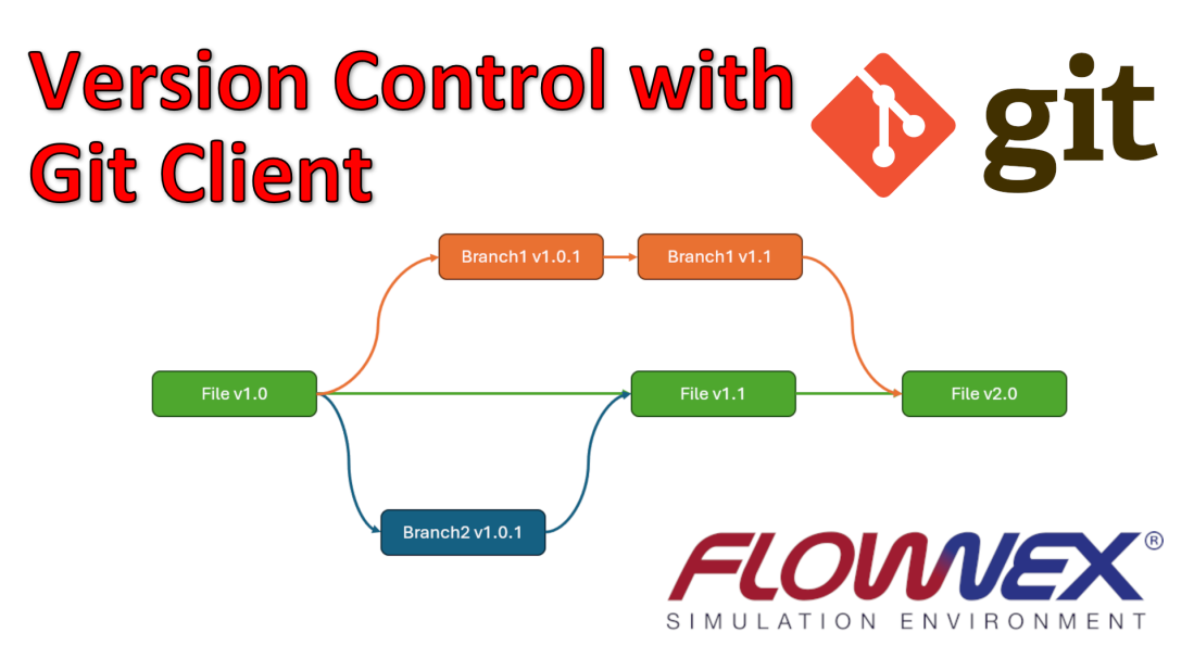
Flownex 2024 has added version control in the form of a Git Client. In Git, all versions of a project and related files are stored in either a local or a remote repository (aka “repo”). This benefits the user as we are able to revert to older versions of a project merge changes made by multiple users, create branches within a design, and capture all changes in a log. The repository can also function as a form of backup.
Accessing the Git Client
There are two ways to access Flownex’ Git client. We can either navigate directly to the executable: C:\Program Files\Flownex SE X.X.X.XXXX\GitClient.exe, or we can open the Git client from the Flownex GUI itself.
To open the GIT client we will want to navigate to the configuration tab in the Flownex GUI and click on “Open Git Client”.
Prerequisites for Setting Up a Local Git Repository
Before we can begin storing versions of our project we want to create a repository. The first thing we must do is specify the Local Repository Credentials found in the settings tab.
The Flownex Git utility automatically records modifications and changes made to a network model. Through the Command History settings, we can omit certain user actions from the recording. Typical exclusions include:
“Open page”
“Deselect all”
“Select”
“Close page”
There is further reading on the settings customizations in section 24.1 of the Flownex General User Manual.
Creating a Git Repository
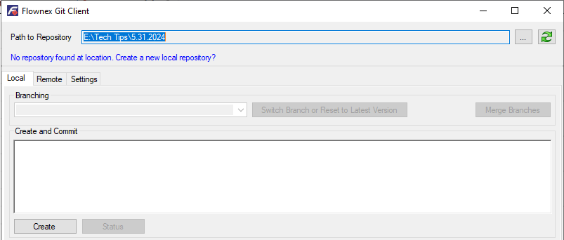
We will want to define our repository directory location in the Path or Repository field found near the top of the Git Client GUI. In this example I use the location E:\Tech Tips\5.31.2024.
If a valid Git repo does not already exist at this location we will click “Create” to make one. A new repo with a master branch will be created and an initial commit will also be performed when we click create.
Committing Changes to Git Repository
Once we’ve defined our GIT repo location we can create and commit the current version of our Flownex network. This can be done by clicking “Save and Commit” in the Flownex GUI in the Configuration Ribbon.
This will save our project and open the Git client. We should see the command history for any changes since the previous commit. At this point we can add any notes and commit our changes to the Git repository. Then we should click “Commit” to save.
Note that if we haven’t already defined our user credentials (found in the Settings tab of the Git Client GUI), we will get an error when trying to commit or create the repository.
Reverting to an Older Version
Through the Git client it is now quite simple to roll back to a previous version of a project.
To roll back to an older version of a project we should first ensure that the Flownex project in question is closed. Next, we will launch the standalone Flownex Git Client
We will need to navigate to our Git repo and then we can simply right-click on the version of the project which we’re reverting to and select “Revert to this Version”.
All changes after the selected version will be reverted without changing affecting the Git log. In this case, I can re-open the project and will see that the inlet pipe length has reverted to it’s original 100 m length.
Additional Operations
Other actions and operations available through the Git Client are described below. We can find more detailed information on these in section 24.2 and 24.3 of the Flownex General User Manual.
Export this Version
Used to export a copy of a selected version of a project.
Create and Switch to Branch
Used to create new version branches within a given master.
Switching between Branches
Users are able to switch between branches for a given project.
Merging Branches
This action will merge changes captured from separate branches into a specified “To” branch.
Add Remote and Push
This function will push existing local repo branches to a remote repo.
Clone
Used to copy a remote repo to a local location.
Fetch and Merge (Pull)
Retrieves changes from a remote repo after a clone or previous fetch.
Push
Updates all locally made changes to the remote repo.
Track Remote Branches as Local
This option allows for tracking a non-master branch from a cloned or fetched remote repo.
In the 2022 Flownex release (8.14.0) a new feature has been added to create Reduced Order Models. Today I’ll go over the basics for creating a reduced order model and how this can be utilized.
To demonstrate this functionality I built a simple network representing a shell and tube heat exchanger. In this model we’ve got liquid water on both the hot and the cold side. For simplicities sake we’ll keep the conditions such that the phase is always liquid.
The ROM builder setup is found under the “Configuration” ribbon in Flownex.
To configure our Reduced Order Model we will want to create a configuration and then define our Inputs (independent variables) and our Results (dependent variables). We do this by dragging and dropping inputs and results into the ROM Builder Configuration Window. For this example the independent variables will be the hot and cold side inlet mass flow rates and temperatures.
We’ll notice there are three different statuses for the ROM configuration. “New”, “SensitivityAnalysisCompleted”, and “NeuralNetworkTrained”. To complete the sensitivity analysis portion we need to set bounds for our independent variables, enter the total number of runs, and then click “Generate and Overwrite”. If we already have started creating our ROM and we simply want to expand the dataset we may want to choose “Generate and Append”.
Flownex will then run the sensitivity analysis which will provide the dataset to train our neural network.
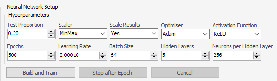
In the creation of the neural network there are a variety of “hyperparameters” which can be adjusted to change the complexity and depth of the model. In this example we will stick with the default values but you can read all about what each of these parameters does in Chapter 23 of the Flownex General User Manual. At this point we can click the button to Build and Train our neural network! In the top right of the ROM Builder window we can see the approximate time remaining.
There are a few graphs we can view in the different tabs to assess the accuracy of our model. I am particularly fond of the results – predicted vs actual. This gives us an understanding, at a glance, of the deviation in what the ROM predicts vs Flownex results.
The last step is to export this as a standalone Functional Mockup Unit (FMU) for use in either other Flownex networks or in another tool like Ansys Twinbuilder.
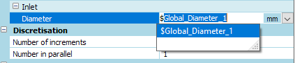
Do you ever find that the units on your Flownex input don’t match what you’re inputting? But you don’t notice until you’ve already typed in the value? There’s a trick to avoid redundant typing! After typing in our input we simply hold CTRLwhile changing the unit.
Here’s what it looks like if we hold Ctrl while choosing a new unit for a diameter input.
If we instead choose the unit while not holding Ctrl we see the units convert automatically.
If you’re more of a keyboard commando and like to avoid mouse-clicks we can also type in the units ourselves.
Some helpful keyboard shortcuts when entering units for areas, volumes, etc…
Often we find ourselves wanting to visualize results in a way to quickly understand how our thermal-fluid system is behaving. This is particularly desired when dealing with thermodynamic cycles. What I’d like to showcase today is how we can use the X-Y graph to plot an Organic Rankine Cycle. In today’s example I am using Flownex version 8.14.0.4675.
Rankine Cycle Modeling in Flownex
I won’t spend too much time on the system model itself, just note that we are working with a very simple network of flow components to lay the groundwork for the example. We use flow resistance elements to build the bulk of the network. We also use composite heat transfer elements to add/remove energy from the fluid. A turbine is used to extract power and, for simplicities sake, rather than model a pump we fixed the mass flowrate on one of the flow resistance components.
Creating the TS Diagram
To create the TS diagram we might first think we should use the Operating Point Plot. While this plot is indeed used for TS diagrams, since we want to plot multiple points we should instead use the XY Graph found in the components library under Visualization > Graphs. The XY Graph can be dragged and dropped onto the drawing canvas.
Another option would be to add the XY Graph as its own page. This can be done by clicking on the Project View pane, selecting the “Graphs” button, then right-clicking on the folder and adding a new graph page.
Then, to add our TS data points, we’ll simply drag and drop the Fluid Data Reference from the key components/nodes in our system onto our newly created graph.
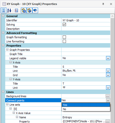
Lastly, if we’d like to connect the data points we can do so by editing the properties of the XY Graph to connect points.
There we have it! A TS diagram with our operational points overlaid all in Flownex! Recall we can expose a lot of additional formatting for our graphs by checking the boxes under Advanced Formatting for either Graph formatting or Line formatting.
We’ve all experienced that fear. When we sit down at our computer and realize that all of our applications are closed. That Windows decided to do a restart in the middle of the night. If we are running any long simulations the thought of having to restart from the beginning is a tough pill to swallow. Luckily, in Flownex, we can use the backtracker functionality to create re-start points during the simulation. In today’s demo I am using the most recent Flownex release, 8.14.0.4675.
Enabling the Backtracker
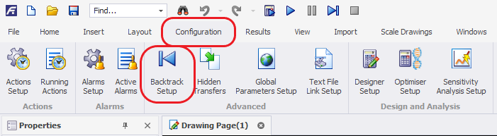
The Backtracker is useful both for resuming long transients and for troubleshooting transient behavior around a transient action. The Backtrack setup can be found in the Configuration ribbon at the top of the Flownex GUI.
After clicking Backtrack setup we will see the backtracker pane available on the right side of the GUI similar to “Snaps”. We will want to click the floppy disk (save) button in the Backtrack pane to enable saving of backtracks. The button will have a blue outline when backtracking is enabled. The “X” button will delete all backtracks.
Backtracker Inputs
In the Backtracker interface we have several inputs we can define. The most important to define are the interval and the count.
Interval
Defines how often a backtrack is saved. The default unit for interval is in seconds.
Count
Determines the count of recent backtracks that are retained in the Backtracker. If we want to capture the entire transient we should multiply the count by interval to make sure the entire duration is covered.
“Use prefix number”
This checkbox along with the “Start number” will save the backtracks with the desired number as a prefix, counting up with each concurrent backtrack save.
“Use snap name as prefix”
This checkbox will ensure that the backtracks saved have the prefix of whatever snap was loaded before the run was initiated.
“Steps after snap load to first backtrack”
This allows us to specify how many timesteps should complete (after initial snap load) before the first backtrack is saved.
Breath Easy and Run Transients
At this point we should be able to run our transient and see the backtracker populate. To load a saved backtrack point we should ensure our simulation is in an inactive state before right-clicking on the backtrack and choosing load. From this point we can resume our transient simulation.
Bonus Tip!
When troubleshooting a transient right-click on the backtrack just before the event and select “copy to snap” so that you can retain and load the state of the network at this start point.
The new 2022 Flownex release is here! Lots of great enhancements to take your simulations to the next level highlighted below.
Major Enhancements
New Non-Iterative Transient Solver
A new non-iterative transient solver has been implemented in Flownex®. Compared to the customary iterative solver, the non-iterative transient solver increases solve speed substantially during transient events by eliminating the need to iterate within time steps. This becomes very advantageous for networks of all sizes, but especially where large systems need to be modelled over a prolonged time span.
The user can switch between the iterative transient solver and the non-iterative transient solver via the dropdown provided in the Transient solver settings category on the Flow Solver input dialogue. For easy access, a direct toggle between the solvers was added as a tab to the Home ribbon as well.
Fig. 1 – Non-Iterative Transient Solver Toggle on the Home Ribbon.
Fig. 2 – Non-Iterative Transient Solver Selection Option in the Flow Solver.
The non-iterative transient solver retains the implicit pressure-velocity coupling in use for the iterative solver, thereby maximizing numerical stability in typical flow systems. Since the pressure-flow solution is not iterated with respect to the enthalpy solution, the method may be classified as semi-implicit.
Instead of using successive iteration with underrelaxation to obtain a converged solution, all governing equations are fully linearized with respect to the primary variables as well as the temporal variable, using exact and accurate gradients and derivatives without any relaxation. For this reason, all inputs within the Convergence, Relaxation Parameter as well as the Iterations categories become redundant when using the non-iterative transient solver option.
Mixture Generalization
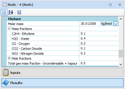
The capability to create a mixture of fluids has been expanded to create mixtures of mixtures for all fluid types, with the exception of two-phase fluids. When a fluid mixture is created, the user now has the option to select more than one liquid and more than one gas when creating mixtures for each of those phases. The below figure shows a Gas and Liquid Mixture, where the user can create a liquid mixture and a gas mixture that consists of multiple liquids and gases within the liquid-gas mixture.
Fig. 3 – Example of a Gas and Liquid Mixture with a Mixture of Gases and a Mixture of Liquids.
Mixing rules for transport properties are applied to the individual phases separately and in the case of a liquid-gas mixture, additional liquid-gas mixing rules are applied when determining the transport properties of the liquid-gas mixture-of-mixtures.
To use the new capability a mixture is configured in the Fluid mixture specification dialog. The remaining user interface experience has not changed. Mixture mass fraction boundary conditions are specified as before, with the list of fluid components expanded to include all of the components of the mixture.
Fig. 4 – Specifying Mass Fractions of a Liquid-Gas Mixture which Contains a Liquid Mixture and Gas Mixture.
Similarly, the result property displays the fluid component mass fraction results for the expanded mixture of mixtures, as seen in Figure 5.
Fig. 5 – Mass Fraction Results of a Liquid-Gas Mixture which Contains a Liquid Mixture and Gas Mixture.
As phase transitions in two-phase fluids are significantly impacted by the presence of other two-phase fluids, the new mixture capability does not currently include the possibility to create a mixture of two-phase fluids. It is however possible to create a Two-Phase Fluid and Gas Mixture where a mixture of gasses can be specified with a single two-phase fluid, as seen in Figure 6.
Fig. 6 – Two-Phase Fluid and Gas Mixture.
ROM Builder
The Flownex® ROM (Reduced Order Model) Builder generates a multi-platform enabled FMU (Functional Mock-up Unit) containing a Neural Network that was trained on sensitivity analysis data. The user is guided from specifying the input and result properties, creating sample data in a sensitivity analysis, specifying the Neural Network hyperparameters, evaluating the trained Neural Network to exporting the FMU ROM using one convenient dialog. The ROM Builder Configuration dialog can be seen in the image below:
Fig. 7 – ROM Builder Configuration.
Fig. 8 – ROM Builder training a Neural Network
Video Recorder
The capability has been added to record graphs and the screen synchronized with transient solving. The video recording options are added to the properties of each graph. When “Record graph as video” is set to “Yes”, a new video is recorded for each transient run. From the Video Recorder task properties (under Solvers), Flownex® can be configured to record the whole screen.
Fig. 9 – Recording a graph to the Videos folder.
Two Phase Heat Transfer
The two-phase fluid generator has been updated to include Steiner and Taborek normalized coefficients and includes an updated radiation model specification. In previous versions the Steiner and Taborek normalized coefficients were effectively hardcoded and were only available for a limited number of two-phase fluids. These coefficients have now been moved to the two-phase fluid data files and the fluid generator therefore required updating to allow the user to provide the appropriate values for generated fluids. The latest two-phase data file format also provides for the selection of the radiation participation model to be used for the generated fluid.
Fig. 10 – Two-Phase Fluid Importer with Saturated Boiling and Radiation Model Specification.
Minor Enhancements
USER INTERFACE FRAMEWORK
Higher resolution (4K) compatibility has been added to the Graphical User Interface.
ACTIONS
The capability to specify a Ramp action has been added. When a Ramp action is created, the user can specify the duration and final value for the action rather than the coefficients for a straight line.
Fig. 11 – Ramp Action.
UNITS
The mils unit has been added that is used for vibration.
Added the capability for a user to reset the unit of a property to the current selected unit system default. This option is available on the context menu on a property, as seen below.
Fig. 12 – Reset Unit Option.
GRAPHS
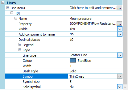
Added a property to change point symbols to be solid or hollow.
Added a ThinCross symbol type.
Fig. 13 – ThinCross Symbol Type and Solid Symbol Option Properties added to Graphs.
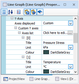
Grouping line items with the same unit group onto one Y-axis is now possible. The “Display multiple Y-Axis” property has been replaced with ”Axes displayed” property.
Fig. 14 – Axes Displayed Property.
Fig. 15 -Axes Displayed Property.
COMPONENT CHARACTERISTIC GRAPHS
An option to view all Angles on Compressor Component Characteristic Graph has been added.
Angles are now available to be checked/unchecked from the graph legend.
All four dimension’s values of the chart are displayed in the chart tooltip.
Only plotting the closest lines functionality is still available by setting a new property: “Show closest background lines” to “Yes”. Property is below “Background lines”.
By default, all lines with check boxes will be displayed for new graphs and graphs from older projects.
SCRIPTING
The Script component has been updated such that the “Initialise” function is called only once before Steady State and “Cleanup” is called once after Steady State. This is done if any or all of the options are active for Before, During and After Steady State. Previously it was called multiple times during Steady State if more than one of the options were active.
The Iterative Script’s “Initialise” and “Cleanup” functions now works similar to a normal Script and is called before and after every steady state and called before and after every transient.
The font of the code editor was changed to a monotype font in order for spacing to align better.
A repository was added that allows for easy sharing of values between scripts. The repository of values can also be loaded and saved as needed.
An application setting has been added so that new pages have the viewport in the middle of the page. This setting is false by default.
Fig. 16 – Viewpoint in Center for New Pages Setting.
SNAPS
Added an application wide setting: “Turn snap before run on by default”. This option is false by default, but a user can make it true, then it will be on for all new projects.
Fig. 17 – Turn Snap Before Run on by Default Option.
PCF IMPORTING
Added a default import mapping that imports components other than only pipes as applicable.
Fig. 18 – Import Configuration Dialog.
DATA TRANSFER LINKS
Implemented bi-directional data transfer capability for Data Transfer Links. The user can drag and drop from the left or the right side of the Data Transfer Link Setup dialog. The direction of the transfer is indicated by the arrows. Bi-directional transfers show arrows at both sides, as seen below.
Fig. 19 – Bi-Directional Data Transfer Capability for Data Transfer Links.
The letters F and C are displayed on a Data Transfer Link when a factor (F) or constant (C) is used.
Fig. 20 – F and C Displayed on Drawing Page.
FLOW PATH GRAPHS
Added the ability to plot Flow Path Graphs along the Rotating Annular Gap length and length increments of the Rotating Channel.
TWO PHASE PRESSURE LOSS
Added output for Lockhart-Martinelli two-phase pressure loss calculations and the parameters that are used in its calculation as results.
HEAT TRANSFER
Reynolds and Prandtl Number results have been added to convective subdivision element results.
Errors have been implemented to prevent Composite Heat Transfer element to Composite Heat Transfer element connection via a solid Node with non-adiabatic boundary conditions, since these are non-physical configurations.
RELAP COUPLING
Added an option to Relap simulation to save every transient step’s output file.
Fixed the problem where the minor edits were deleted in Relap files.
Allow users to add additional inputs or outputs to the Flow solver coupling. This is especially useful to extract additional results from the Relap simulation.
COMMAND LOGGING
Flownex® logs many of the user actions now to a file. This log is useful to keep track of what was changed in a project and when.
The command log files are located in the project folder in the sub folder CmdRec\Logs.
Each new Flownex® session starts a new log with the date and time of the session. The user, operating system and computer name are recorded at the top of each file.
The following user actions are recorded to the file:
Interaction with the drawing canvas (e.g. adding, deleting, selecting components).
Interaction with pages (opening, closing, selecting pages).
Exported Flownex® FMUs now launch a separate console that communicates with the Flownex® instance that is launched. This is done to enable the FMU binary to be unloaded by the master simulator. The binary was previously locked until the master simulator process shuts down due to the CLR being loaded as part of the binary. All CLR code is now loaded in the separate console process.
The locked binary gave a warning or error when the FMU was unloaded, even though the FMU functioned correctly.
NIST IMPORTER
The NIST fluid importer was updated to list all the available fluids and mixtures in NIST.
BUG FIXES
RESULT LAYERS
Fixed the bug where Result Layers did not update during transient in 3D view.
Result Layers are now updated after a Snap is loaded.
Fixed absolute value usage in Result Layers.
Changed mass flow, volume flow and velocity built in Result Layers to use absolute values.
VELOCITY PID
Fixed the bug where state of the PID was not saved to Snaps.
DRAWING TEXTS
Fixed the problem when pressing the Cancel button when changing settings for the drawing texts, the operation was not fully cancelled.
EXCEL COMPONENT
Fixed bug where Snaps were not correctly loaded for Excel component if an editor wasn’t opened previously or network wasn’t solved previously.
RESULTS OVERVIEW
Fixed the bug where the Solving On/Off state was not saved with the project. This meant that the user had to turn it off again every time the user opened a project.
API
Fixed a bug where an exception in the user interface was sometimes shown when using the API. This happened when using the API with a network with open graphs.
DUCTING
Added tooltip results for all Junction component types.
POSITIVE DISPLACEMENT PUMP
Fixed the unit for NPSH in the characteristic chart.
EXCESS FLOW VALVE
Added tooltip results for the Excess Flow Valve.
NODES
Fixed the error where a user could connect multiple views of a node or element to a fiber that should only allow a single connection. This caused an error in the solver that was not very descriptive and hard to trace.
WARNINGS AND ERRORS
Updated MATRIX_NOT_POSITIVE_DEFINITE error to also show the Node related to the error.
Added a warning when a large non-normalized energy residual is detected at a node and the energy equations may not have converged.
NEUTRONICS SCRIPT
Implemented Total power result and Transient Fix power option correctly for the Neutronics Script.
Initialisation was not correctly called for the Neutronics Script and a Cleanup function has been added.
BOUNDARY CONDITIONS
If Mass source fraction is disabled after being specified, the mass fraction did not reset to 1 and 0, as with the normal mass fraction specification.
Fixed the problem where a Data Transfer Link could write and change the temperature of a Boundary Condition even if the option to specify temperature is not turned on.
HEAT TRANSFER
Addressed Conduction results that went out of sync when changing from upstream Convection results to Conduction element results after an increment other than 1 is selected for the upstream Convection results.
TWO PHASE FLOW HEAT TRANSFER
The Steiner and Taborek reference coefficients are now specified in the two-phase fluid specification file and are no longer hard coded. Approximations have been provided for Flownex® fluids that are not featured in the original Steiner and Taborek paper, and a warning is issued.
The heat flux at the critical heat flux conditions is used when the wall temperature commensurate with the critical heat flux that is calculated. Previously the current heat flux result was used in the wall temperature calculation.
Updated the Groeneveld critical heat flux and film boiling lookup tables to the latest versions.
V&V
The Validation Runner was renamed to Verification Runner. The Verification Runner is now included in the Nuclear module and uses the normal Nuclear license and does not require a separate license anymore.
ACTIONS
Fixed the problem where actions wrongly set integer values at the start of an action. The initial value of the integer property was always added as an offset. This was reported as a multiplexer problem but is a general problem.
See how Flownex, ADT TurboDESIGN, and Ansys can be used to expedite and optimize turbopump design for propulsion systems in this joint webinar presented by PADT and ADT.
Hi All! It has been a little while since a Friday Tech Tip has gone out – 2022 has been a busy year so far! Today we’ll share a quick how-to on using the property monitor to interrupt our simulations. This is a powerful tool for transient analysis to quickly define a pause or stop criteria.
In this demo we’ll be reviving the previous fire suppression demo. I’m faced with a situation where I don’t know how long it will take for the suppression agent bottle to empty. Rather than running a long simulation or trying a variety of transient lengths we can instead use the property monitor to interrupt the solve.
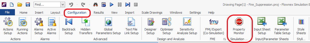
The property manager can be found in the configuration ribbon;
The important thing here is that we pick a reasonable property to use as our criteria for interrupting the solve. My first thought was to pick the pressure remaining in the tank but after giving it more thought I think that mass flowrate is probably a better measure since it may take quite awhile before the pressure in the tank drops all the way down to atmospheric.
To assign a property to monitor we simply drag and drop the property into the property monitor window:
There are a lot of settings we can manipulate in the property monitor for a variety of different applications. In this instance, I would like the solve to pause when the mass flow rate drops below a certain point. We can do this by checking the “Pause” box and choosing an appropriate criteria to trigger the pause.
Once this is set up we can safely let the simulation run unattended, safely knowing when our pause criteria is met Flownex will interrupt the solve for us!