Often we find ourselves wanting to visualize results in a way to quickly understand how our thermal-fluid system is behaving. This is particularly desired when dealing with thermodynamic cycles. What I’d like to showcase today is how we can use the X-Y graph to plot an Organic Rankine Cycle. In today’s example I am using Flownex version 8.14.0.4675.
Rankine Cycle Modeling in Flownex
I won’t spend too much time on the system model itself, just note that we are working with a very simple network of flow components to lay the groundwork for the example. We use flow resistance elements to build the bulk of the network. We also use composite heat transfer elements to add/remove energy from the fluid. A turbine is used to extract power and, for simplicities sake, rather than model a pump we fixed the mass flowrate on one of the flow resistance components.

Creating the TS Diagram
To create the TS diagram we might first think we should use the Operating Point Plot. While this plot is indeed used for TS diagrams, since we want to plot multiple points we should instead use the XY Graph found in the components library under Visualization > Graphs. The XY Graph can be dragged and dropped onto the drawing canvas.

Another option would be to add the XY Graph as its own page. This can be done by clicking on the Project View pane, selecting the “Graphs” button, then right-clicking on the folder and adding a new graph page.

Then, to add our TS data points, we’ll simply drag and drop the Fluid Data Reference from the key components/nodes in our system onto our newly created graph.

Lastly, if we’d like to connect the data points we can do so by editing the properties of the XY Graph to connect points.
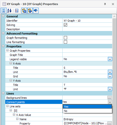
There we have it! A TS diagram with our operational points overlaid all in Flownex! Recall we can expose a lot of additional formatting for our graphs by checking the boxes under Advanced Formatting for either Graph formatting or Line formatting.

