Tag: simulation
Optimizing Engineering Workflows for Propulsion System Design
See how Flownex, ADT TurboDESIGN, and Ansys can be used to expedite and optimize turbopump design for propulsion systems in this joint webinar presented by PADT and ADT.
Creating a Custom Fluid in Flownex

Flownex Tech Tip #6
Occasionally glossed over, adding custom fluids is a fairly standard operation in Flownex that we don’t think about until it’s necessary. There are a couple of ways to do this which we’ll go over in today’s post. I am working in Flownex 8.12.7.4334.
Creating a mixed fluid
To create a mixed fluid we first need to create a folder for this fluid in our project database. This can be done in the charts and lookup tables pane by right clicking on “mixed fluids” and selecting “add category”. We can create our new fluid by right-clicking on the new folder and selecting “Add a new mixed fluid”. Note we can right-click and rename both the fluid itself and the containing folder.
To define our new mixed fluid we double-click on the new mixed fluid to open the editor. Here we can add the components of our mixed fluids.
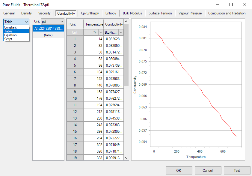
Creating a new fluid from scratch
To create a fluid from scratch we repeat the same process of creating a folder and creating a new fluid as above with the exception being that we’d complete these steps under the “Pure Fluids” category. Once this is done we’ll need to double-click or right-click > edit our from scratch fluid and enter in the fluid properties. Note for many properties we can define the relationship with pressure and temperature as constant (non-dependent), table, equation, or script.
Importing a fluid
To import a fluid we will follow the same steps of creating the folder under pure fluids. Now instead of right-clicking and adding new we will right-click and select “import”. Then we simply navigate to our desired fluid file and click “Ok”.

Bonus Tips!
- In the window where you define your fluid you’ll notice the “Test” button. This feature can be utilized to test created fluids to confirm properties against known properties for given pressures and temperatures.
- We can also copy and paste fluids from the master database into the project database to give us a good starting point for creating similar fluids (or extending properties to higher/lower temps/pressures).
Custom Result Layers in Flownex

Flownex Tech Tip #5
The result layers in Flownex have evolved quite a bit over the last few iterations of the code. Although we might typically associate color-gradient results more with 3D CFD, it does have a place in 1D system modeling. Taking advantage of results layers in Flownex can give a very quick understanding of what is going on with our system, and, with a little customization, can be incredibly powerful as an addition to our design and analysis toolbelt. In this post I am using Flownex version 8.12.7.4334.
How to create a result layer
To create a custom result layer we must navigate to the results ribbon and select result layer setup.

First we want to right-click in the Result Layers window and add a new result layer.

There are two options to add the schema for our result layer. The first is to right-click on the Selected Result Layer Schemas and add either a specific or generic schema. The second, and my PREFERRED, method is to simply drag and drop results from components on the canvas into this window:

Note that I want to multi-select any component types which will be included in this result layer. This could be any flow components which share a common result such as “quality”. I also convert to generic because I want the result layer to apply to all pipes, not just the pipe I initially drag and drop the property from.
Defining the custom result layer
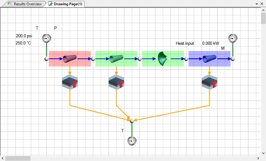
In this example I have a two-phase water network with a cold external temperature. I want to create a result layer to quickly see if the water is in the gas phase, liquid phase, or somewhere in-between. The problem I have been tasked with solving is ensuring that the water never condenses. I will need to determine where we may need to add additional heat flux to the network.
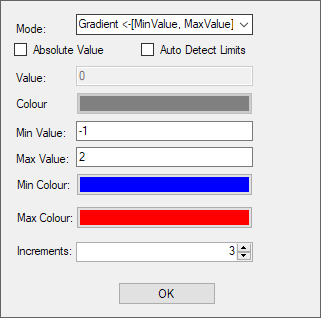
We can use the Quality result property to determine the phase of our fluid. Quality < 0 indicates fully liquid, quality between 0 and 1 indicates liquid/gas mixture, greater than 1 indicates fully vapor.
To make this work as intended I can set up a gradient with three increments going from -1 to 2. The idea being the lowest increment would encompass -1 to 0, middle increment would be 0 to 1, and the top increment would be 1 to 2. For the gradient mode I made sure to pick <-[MinValue, MaxValue]-> so that the max and min increments would extend past the specified range.
As we apply this to our network we can easily see that we do, in fact, have a phase change from gas at the inlet, to mixture in the second two component, to fully liquid near the outlet.
I may decide to add a heater to our outlet pipe and perhaps a thicker insulative layer to all three to attempt to keep the water in gas phase throughout the system.

Bonus Tip!
- Result layers can also be super handy when troubleshooting to quickly identify large pressure differentials, choking points, or other outlying fluid properties.
Input Sheet Hacks in Flownex

Flownex Tech Tip #3
Building on last week’s global parameters example I’d like to show some tricks within the input sheet environment. These are really more so excel tricks – but the methodology within Flownex is slightly different. In this example I am working in Flownex Version 8.12.7.4334
Refresher on using Input Sheets
To create a new Input Sheet we will navigate to the project tab, then select “Excel Reports/Pages”, right-click on the Input Sheets folder, and select “New Input Sheet”

To add inputs to the sheet it’s as simple as dragging and dropping the inputs from the component into the desired cell in the Input Sheet.
Formatting our Input Sheet
I like to use color, shading, and border to specify which cells contain inputs so that if I pass the project off to a client or colleague it is immediately clear what variables they should be editing and which cells they shouldn’t change.
To modify the formatting we need to enter “workbook designer”. This is done by right-clicking on the input sheet and selecting “workbook designer”
All of the standard Excel-type formatting is available here, including adding graphs, images, etc. Typical operations are found in the format menu on the top ribbon.
Drop Downs
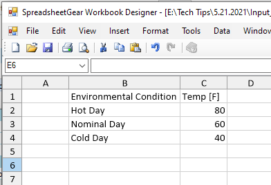
A more advanced Excel operation I like to integrate into these types of input sheets is a drop-down where multiple inputs may be tied to a given condition. In the example below I set up a scenario for given ambient temperature for cold day, hot day, and nominal day.
In the workbook designer we will click “insert” > “worksheet” and build our list of environmental conditions. On the right we will set the associated temperatures.
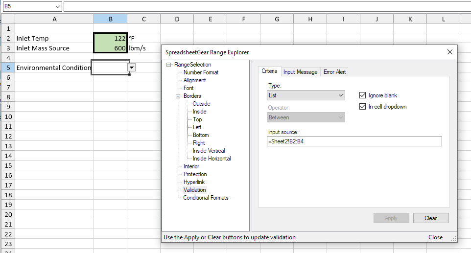
Back on Sheet1 we will need to set up the data validation cell reference to this table. Select the cell where we want to add the dropdown and go to data > validation. We will choose list, and reference cells B2:B4 of Sheet2.
We will need to use VLOOKUP to associate the temp to another cell based on this dropdown. Where this becomes valuable is when we have many input variables tied to each of the dropdown selections.
In this example, since we’ve put the applicable temps a single column to the right the syntax for VLOOKUP will be “=VLOOKUP(B5,Sheet2!B2:C4,2,FALSE)”. After this is added it should behave as follows:
As I mentioned before, this trick becomes very powerful when you have many different environmental or operational inputs tied to a single “scenario” that you want to model in an individual run rather than in a parameter study.
Bonus Tip!
- All of these tricks can be applied to any of the excel-type sheets within Flownex. Remember to be careful with parameter tables as the inputs and results are tied to the columns instead of individual cells.
Working with Global Parameters in Flownex!

Flownex Tech Tip #2
As we build more and more networks it quickly becomes tedious to enter in the same inputs many times. There are a couple methods of using global parameters to save us lots of time and clicks. In this example I am working in Flownex Version 8.12.7.4334
Refresher on Global Parameters
Global parameters are just what they sound like. Parameters defined globally for the project. These could be any type of component input; diameter, length, temp, pressure, etc.
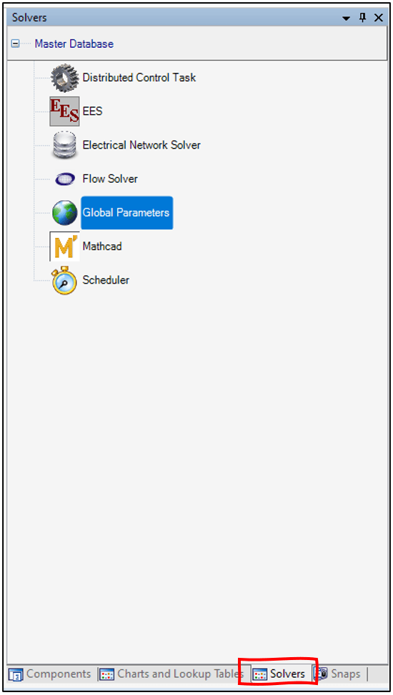
The global parameters can be found in a couple of locations. Under the configuration ribbon we can open the global parameters in a floating window which gives us a friendly interface for creating or modifying these parameters. To create a global parameter one may simply right-click in the GlobalParameters window and select Add (hint: there’s a better way!).

Global parameters can also be accessed in via the solver tab in a similar way to typical inputs (this is important later on).

The Quick way to add Global Parameters
We don’t really want to have to navigate to that configuration ribbon, right-click a bunch, choose names and assign units do we? Good news! There is a much faster way to add a global parameter. We can add a global parameter with minimal work by simply typing a dollar sign “$” prefacing the name of the tag in any of our component input fields! Remember to hit enter after typing the identifier.
Once a global parameter has been defined we can tie more inputs to the existing parameter by typing the dollar sign “$” and choosing the correct parameter from a drop down:

As you can see, this can be quite a time saver when building a network! The next trick utilizing global parameters will have to do with using them for actual analysis.
Using Global Parameters as Manipulatable Inputs
The default/slow way to change a global parameter would be to go to the configuration ribbon > global parameters, and manually change the value in the floating window. No thanks. This is not automated at all and requires many clicks.
The better way to utilize the global parameter as an input would be to tie the global parameter to an input sheet, parameter table (for a parametric study), or even a human machine interface component (HMI).
Global Parameters in Input Sheet
For a design variable that an analyst or engineer may change which would then remain constant (such as pipe diameter) the input sheet comes in very handy. To reference a global parameter in the input sheet recall the second method to access the global parameters and then simply drag and drop onto the input sheet:
Global Parameters in Parameter Table
If you are trying to run a parametric study where you are varying something like ambient temperature, it makes sense to use a global parameter as you may have many boundary conditions defined by a single global parameter. Similar to the input sheet this can be tied to a global parameter by a simple drag and drop operation:

Global Parameter in a Human Machine Interface
By now I expect you are catching on. The trick to defining a global parameter externally is to use the second method; solver tab > global parameters, and then drag and drop to your desired connection. In the HMI instance I’ve tied inlet mass flow to a Track Bar so that a user can dynamically change the flow rate during the solve:

Global Parameters are efficient and POWERFUL
We can use global parameters during network construction using the “$” shortcut to build our networks much more quickly and keep identical inputs the same. We can tie these global parameters to other tools to keep our user inputs all in one place, reducing clicks, and reducing the chance of forgetting to update an input.
Bonus Tips!
- Global Parameters can also be used in Designer so that you can keep your independent to dependent variable count the same (EX: Adjusting ALL pipe diameters to target a single exit flowrate)
- Global Parameters can be adjusted via transient actions (EX: Adjusting ambient temperature to model the changing temperature over the course of 24 hours).
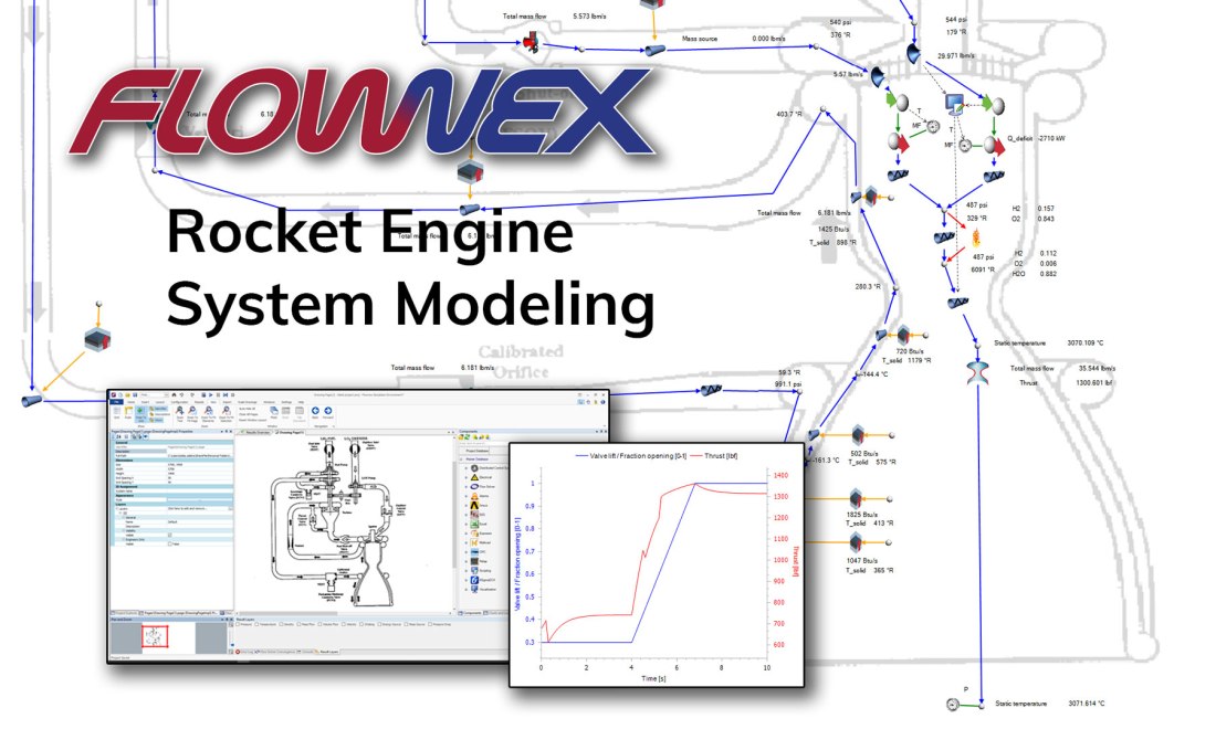
Building a System Model of the RL-10 Rocket Engine in Flownex
When we engineers are building a new system or iterating on an existing design it can be expensive. Simulating a full system level model in a 3D CFD program can take days. Making iterative changes to an existing system can be costly or even impossible. Utilizing a one-dimensional system modeler like Flownex allows us to analyze many different designs very quickly, on the order of seconds or minutes.
Flownex is a thermal-fluid network modeler. It is a simulation tool that allows for 1D fluid modeling and 2D heat transfer. It uses a variety of flow components, nodes, and heat transfer elements to model the entire system we are interested in analyzing. It solves conservation of mass, momentum, and energy to obtain the mass flow, pressure, and temperature of fluids and solids throughout the complete network. Because of this approach we can analyze large, complex networks very quickly, iterate on designs, and even run short or long transient simulations with ease.

In the example today we are looking at a version of the RL-10 rocket engine, which has been a staple in the delivery of satellites into orbit and an essential part of many spacecraft. The specific iteration of the RL-10 we will be using for building our network model is the RL10A-3-3A. A good place to begin with any system model is a system schematic:

In Flownex we can assign an image (could be from a P&ID diagram, a CAD cross-section, or even a satellite image!) as the background for our drawing canvas. We simply need to right-click on the drawing canvas and select Edit Page to bring up the drawing canvas properties.

Clicking on the action button under Appearance > Style brings up the Styles Editor. Here we can change the fill style to Image and select the appropriate image for our background.

In the case of the RL-10 we can use the image from figure 2 as our background image. We may want to consider adjusting the opacity of the image so that it blends into the background a little bit more.

In Flownex building a system model is as simple as drag and drop. We can build our rocket engine using a variety of flow components from the Flow Solver library. To build the RL-10 system model we will be using the following components:

CEA Adiabatic Flame component to model combustion.
Composite Heat Transfer component to model thermal transport through pipe-walls to ambient and to model the regen.
Boundary Conditions to constrain our system at the inlets and outlet.
Basic Valves to model the different valves in the system,
Flow Resistances to model specified losses where appropriate.
Flow Interfaces to model the fluids entering the combustion chamber (to transfer fluid properties as we switch from two-phase O2 and H2 to gaseous fluids for modeling combustion.
Pipes for modeling various flow-paths.
Restrictors with Discharge Coefficient for our injection ports to the combustion chamber.
Restrictors with Loss Coefficient to model both the Calibrated Orifice and the Venturi contraction/expansion.
Basic Centrifugal Pumps for our Fuel and LOX pumps.
Simple Turbine to model the Fuel Turbine
Shafts to connect our different pumps mechanically.
Gearbox is used to connect the shafts between the LOX pump and the Fuel Pump.
Exit Thrust Nozzle to determine total thrust.
A Script is used in assigning O2 properties prior to combustion.
The components may be dragged and dropped from the component library onto the drawing canvas to build our system model. We can also copy and paste components that are already on the canvas into different locations. This can be especially useful when the same inputs for say, a pipe, are used consistently throughout the model. All components have both Inputs and a Results associated with them as seen in the figure below. This is how we will define our flow components.

The completed model of the RL-10 Rocket Engine can be seen below. There are a few simplifications; we are using composite heat transfer components to model free convection to a specified ambient temperature (as though this was a land-based test). Rather than tie the actual temperatures and flow conditions in the nozzle to the regen we are using assumed temperatures and convective heat transfer coefficients. For additional fidelity we could model the heat transfer between these two flow paths with calculated convective heat transfer coefficients and we could model cross-conduction along the pipes which deliver the fuel and oxidizer to the combustion chamber. With additional effort, more complex use cases could also be simulated.

For the sake of demonstration we set up a transient action to slowly vary the oxidizer control valve fraction open; starting at 30% and ending at 100% open and observer the change in thrust at the nozzle as a function of this changing transient action.

Plots may be easily added by dragging a Line Graph from the Visualization > Graphs section of the component library onto our canvas. To choose the characteristics we would like plotted against time we simply need to drag and drop the desired inputs or results onto our newly placed line graph.

We can plot both the oxidizer control valve fraction open and the thrust versus time to observe the thrust reaction to the opening of the valve. The thrust plot has some jumps that are likely due to numerical singularities – with additional work this could be improved.
As can be seen, setting up complex system models in Flownex is relatively simple with most operations being drag and drop. For ease of sharing models with colleagues or customers adding a background image makes it very easy to see how the flow components in the model correspond with a system schematic. Setting up and plotting the effects of operational transients is a breeze!
For more information on Flownex please reach out to Dan.Christensen@padtinc.com.
Travel Trailer Analysis in ANSYS Discovery

ANSYS Discovery is a wonderful tool for fast and first look structural, fluid flow, and thermal simulations. Discovery gives us the ability to modify geometry very quickly within the interface and to add or remove features to view realtime simulation reactions. This allows us to quickly iterate, explore design changes, and better understand interaction between our design and the environment. Today we are going to be investigating the pressure profile on the exterior of a travel trailer being pulled behind a truck down the highway.

In this analysis we are using a 2018 Chevy Silverado 2500 model pulled from GrabCAD with a generic 25 foot travel trailer. Based on described experience we’ve noticed that the roof and sidewalls of a moderately sized travel trailer seem to bow outwards at highway speeds near the front of the trailer. The first thing to do is to put this model in an enclosure and prescribe a flow condition at the inlet and a pressure boundary at the outlet. Modeling the truck/trailer combo at a speed of ~55 mph (25 m/s) confirms that there is suction (negative pressure) present in these key areas:

While the actual roof and sidewall separating could be attributed to poor manufacturing processes we wonder if there could be a design change to minimize negative pressure/suction. One idea would be to incorporate some sort of turbulator to break up the laminar flow. I’ve seen turbulator tape in a zig-zag pattern used in aviation for this specific purpose so we’ll try recreating the travel trailer equivalent and see how it goes.
I started with a zig-zag pattern about 4″ tall on top of the trailer to see if I could “pop the bubble”

This did have the intended consequence and it was curious to see how much impact the turbulator on top of the trailer had on the negative pressure at the sidewall of the trailer:

The next thing I wanted to try was moving the turbulator forward or backward to see the effects. Moving the turbulator towards the aft of the vehicle has limited effects but moving it to different locations within the suction “bubble” seems to effect our -500 Pascal isosurface:

This would seem to indicate the presence of a “sweet spot” for turbulator location that merits further research in either the “Analyze” mode within Ansys Discovery or within Ansys Fluent.
Before I hang up my coat I’d like to investigate one alternate design that I’ve seen more often in automotive applications. I’m going to try adding vertical pillars and see how that goes:


We can easily change the height and position of the pillars to see the resultant effects on the pressure isosurface. The pillars also have a significant effect on the suction bubble but I notice that it has less effect on the suction on the sides of the trailer.

Using Discovery we can quickly and easily iterate on designs, get a first-view of the physics, and determine which change or design merits further investigation. In this analysis we can see that there is most definitely a suction profile at the front of a generic travel trailer. If the suction proves damaging we can see that there are several design changes which will help to mitigate this effect.
For more information on ANSYS Discovery please reach out to info@padtinc.com
