See how Flownex, ADT TurboDESIGN, and Ansys can be used to expedite and optimize turbopump design for propulsion systems in this joint webinar presented by PADT and ADT.
Tag: 1D
Modeling a Fire Suppression System in Flownex
Flownex Friday Tech Tips!
Today I’m going to go through my workflow of modeling a fire suppression system in Flownex. This particular system is designed with an aircraft in mind. We’ll go over typical workflow and transient setup using Flownex version 8.12.8.4472
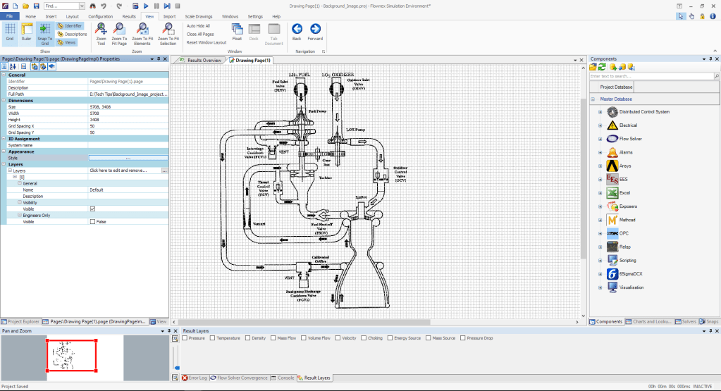
Background Image
See my post on adding a background image for in-depth step-by-step direction. I first set up a background image so I have an easily understood flow schematic to reference in my Flownex build. This also is particularly useful when showing or passing the network off to a colleague or customer who may not have intimate familiarity with Flownex. The image I used in this demo is from this paper by Jaesoo Lee.

Choosing the Appropriate Flow Components
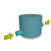
In this model I’ve got a storage bottle, a distribution pipe, and some injection nozzles. I know that I want this to be able to handle two-phase and I know I am pressurizing the bottle with N2 so I will use the Container Interface components to represent the bottle. I will use pipe components for the distribution line, and for the nozzles I will simply use restrictors with discharge coefficients.

Container Interface – Top
Container Interface – Bottom

Pipe
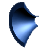
Restrictor with Discharge Coefficient
Building network of components and entering geometry
While building this network I realized I was missing one additional component. I needed to add a valve to open the bottle and release the fire suppressant (HFC-125) and a valve representing a vent to the top portion of the tank which we will leave fully closed.
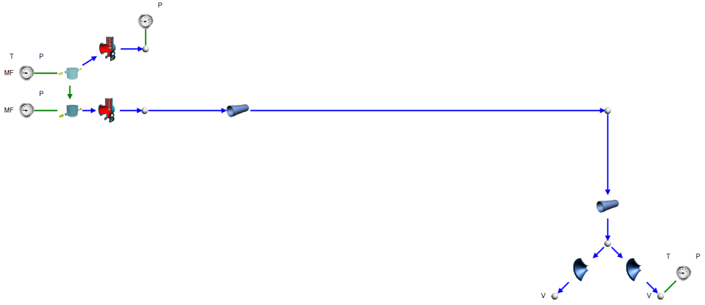
We need to specify our initial pressures, mass fractions, and a temperature on the storage bottle. We also need an outlet pressure and temperature to fully constrain our model. I use a “view” node on my nozzle so that I only need to specify a single outlet boundary condition.
Transient setup
For this transient analysis I am going to open the valve and see how quickly the suppressant discharges from the system. The first thing we will want to do is to remove any boundary conditions that we want to be “free” during the transient. I’ll remove all of the boundary conditions at the storage bottle so that Flownex will calculate the remaining pressure as our system discharges.
I also need to specify our timestep and simulation length. We can do this under the Scheduler properties which can be found in the Solvers pane on the right side of the GUI. I chose a timestep size of 20ms and a total simulation duration of 2 seconds.
Solve Steady State, Snap and Run!
To get a stable transient simulation it’s best to start from a converged steady state. At this point I’ll solve steady state, addressing any warnings that arise. Then we will want to save a Snap of the solve (so that we can load the snap to get back to initial conditions for any future transient runs).

At this point we should be good to run our transient analysis! I’ve added a plot of the pressure in the bottle and pressure just before the nozzles vs time to this project as well:
Sizing Pumps and Manually Specifying a Pump Curve in Flownex

Flownex Tech Tip #12
As a System Engineer you may not always already have equipment decided on for your particular network. Flownex makes it easy to start from scratch and will help determine the equipment necessary to meet the flow or process requirements. In today’s tip we’ll go over how to size a pump using the basic centrifugal pump component and how to manually enter pump curve data. We are using Flownex version 8.12.7.4334
Sizing a Pump
In our example scenario let us pretend we are sizing a pump for a cooling water circuit. We are tasked with finding a pump which will deliver water at a rate of 1 kg/s to the heat exchanger. We know our upstream and downstream boundary conditions as well as the heat added at the exchanger and the speed at which we will be operating the pump.
Choose the appropriate flow component
There are a few different pumps available in Flownex:

Basic Centrifugal Pump: Used when we do not have a pump chart available, particularly useful when sizing a pump.

Fan or Pump: Used when a pump chart is available for modeling either compressible or incompressible flows.

Positive Displacement Pump: Used for modeling rotary and reciprocating pumps where the fluid is incompressible, non-Newtonian, or a slurry.

Variable Speed Pump: Similar to the Fan or Pump but with the ability to interpolate between fan/pump curves for different speeds of rotation.
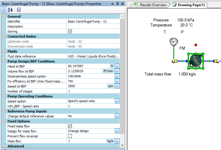
In this case we’d choose the Basic Centrifugal Pump. This is found in the component pane under Turbos and Pumps. Since we only know the RPM we can enter it in the inputs under Speed at BEP:

Recall we don’t know what the design of the pump will be. Since all we know is that the mass flow rate needs to be 1 kg/s we will check the box for fixed mass flow and then select to change design to target our desired flowrate.

Once we hit solve our pump design inputs will be populated such that our desired mass flow rate is achieved. We can cross-reference these values with available pumps to choose the appropriate component for our network!
Specifying a Pump Curve
If we already know which pump we are using, or perhaps are trying to decide between several available pumps, we may need to add these pump curves to Flownex. To add a pump curve we will navigate to the Charts and Lookup Tables pane > Project Database > Flow Solver > Turbos and Pumps. In this scenario we are looking at a single speed pump so we will right-click on Pump and Fan Charts and Add a Category.

We can name our category whatever is appropriate and then right-click on the newly created category to add our own pump chart.

To edit the newly created pump chart we can either double-click on it or right-click and select edit. Now we simply specify the Reference Density and then fill out the table with the relevant data points. To speed things along we can copy and paste a table of data points from excel or whatever source we get this curve from. Don’t forget to check your units!

Bonus Tip!
- Don’t forget you can save created pump charts in a shared database (see previous blog post on creating a shared database)
Creating a Custom Fluid in Flownex

Flownex Tech Tip #6
Occasionally glossed over, adding custom fluids is a fairly standard operation in Flownex that we don’t think about until it’s necessary. There are a couple of ways to do this which we’ll go over in today’s post. I am working in Flownex 8.12.7.4334.
Creating a mixed fluid
To create a mixed fluid we first need to create a folder for this fluid in our project database. This can be done in the charts and lookup tables pane by right clicking on “mixed fluids” and selecting “add category”. We can create our new fluid by right-clicking on the new folder and selecting “Add a new mixed fluid”. Note we can right-click and rename both the fluid itself and the containing folder.
To define our new mixed fluid we double-click on the new mixed fluid to open the editor. Here we can add the components of our mixed fluids.
Creating a new fluid from scratch
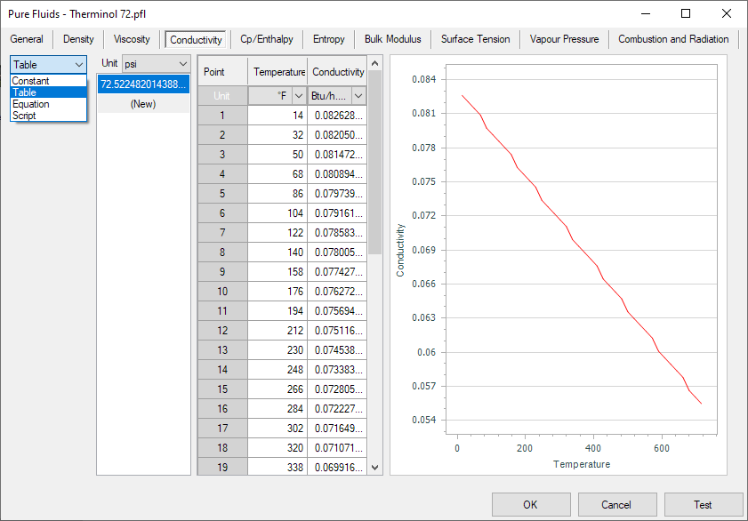
To create a fluid from scratch we repeat the same process of creating a folder and creating a new fluid as above with the exception being that we’d complete these steps under the “Pure Fluids” category. Once this is done we’ll need to double-click or right-click > edit our from scratch fluid and enter in the fluid properties. Note for many properties we can define the relationship with pressure and temperature as constant (non-dependent), table, equation, or script.
Importing a fluid
To import a fluid we will follow the same steps of creating the folder under pure fluids. Now instead of right-clicking and adding new we will right-click and select “import”. Then we simply navigate to our desired fluid file and click “Ok”.

Bonus Tips!
- In the window where you define your fluid you’ll notice the “Test” button. This feature can be utilized to test created fluids to confirm properties against known properties for given pressures and temperatures.
- We can also copy and paste fluids from the master database into the project database to give us a good starting point for creating similar fluids (or extending properties to higher/lower temps/pressures).
Custom Result Layers in Flownex

Flownex Tech Tip #5
The result layers in Flownex have evolved quite a bit over the last few iterations of the code. Although we might typically associate color-gradient results more with 3D CFD, it does have a place in 1D system modeling. Taking advantage of results layers in Flownex can give a very quick understanding of what is going on with our system, and, with a little customization, can be incredibly powerful as an addition to our design and analysis toolbelt. In this post I am using Flownex version 8.12.7.4334.
How to create a result layer
To create a custom result layer we must navigate to the results ribbon and select result layer setup.

First we want to right-click in the Result Layers window and add a new result layer.

There are two options to add the schema for our result layer. The first is to right-click on the Selected Result Layer Schemas and add either a specific or generic schema. The second, and my PREFERRED, method is to simply drag and drop results from components on the canvas into this window:

Note that I want to multi-select any component types which will be included in this result layer. This could be any flow components which share a common result such as “quality”. I also convert to generic because I want the result layer to apply to all pipes, not just the pipe I initially drag and drop the property from.
Defining the custom result layer
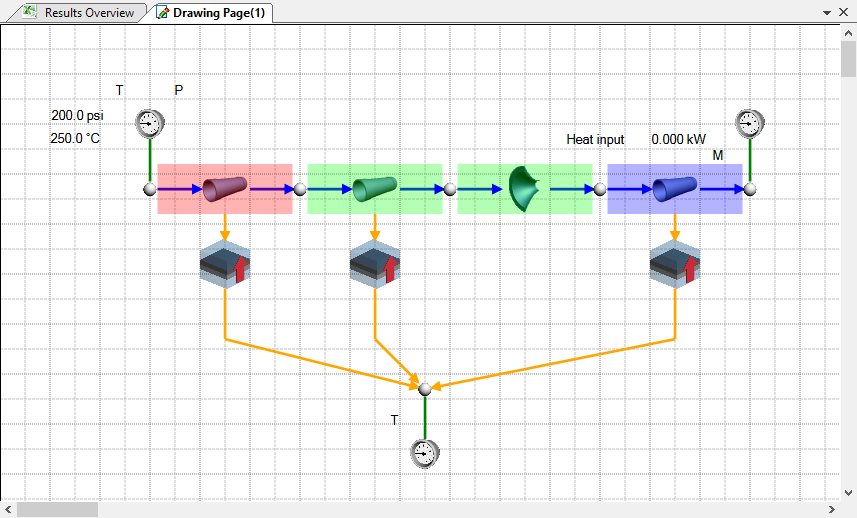
In this example I have a two-phase water network with a cold external temperature. I want to create a result layer to quickly see if the water is in the gas phase, liquid phase, or somewhere in-between. The problem I have been tasked with solving is ensuring that the water never condenses. I will need to determine where we may need to add additional heat flux to the network.
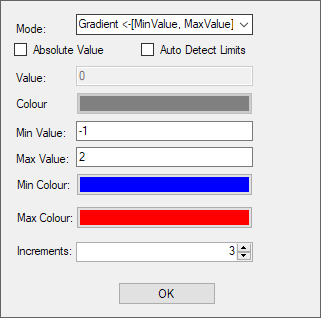
We can use the Quality result property to determine the phase of our fluid. Quality < 0 indicates fully liquid, quality between 0 and 1 indicates liquid/gas mixture, greater than 1 indicates fully vapor.
To make this work as intended I can set up a gradient with three increments going from -1 to 2. The idea being the lowest increment would encompass -1 to 0, middle increment would be 0 to 1, and the top increment would be 1 to 2. For the gradient mode I made sure to pick <-[MinValue, MaxValue]-> so that the max and min increments would extend past the specified range.
As we apply this to our network we can easily see that we do, in fact, have a phase change from gas at the inlet, to mixture in the second two component, to fully liquid near the outlet.
I may decide to add a heater to our outlet pipe and perhaps a thicker insulative layer to all three to attempt to keep the water in gas phase throughout the system.

Bonus Tip!
- Result layers can also be super handy when troubleshooting to quickly identify large pressure differentials, choking points, or other outlying fluid properties.
Adding a Background Image in Flownex
I’m going to attempt to write a recurring blog post on Fridays with tips and tricks in Flownex that I have discovered over the years. This post will be the first of many! If you enjoy please subscribe.
Flownex Tech Tip #1
In this post I will go over what is usually the first step in any network I build. Adding a background image not only helps me lay out my network but also helps colleagues and clients understand networks at a very quick glance. In this example I am using Flownex version 8.12.7.4334
Choosing an Appropriate Image
The first thing we want to do is to make sure that the image size is such that it’s reasonable in size both resolution-wise (so it doesn’t appear pixelated), and right-size so that components don’t appear too small when placed on top. I recommend something in the multi-thousands of pixels both in width an height. 3000 pixels at a minimum. I usually shoot for around 10,000 wide by 5,000 high if the background image will be landscape. For very complex, large networks, it may make sense to go much larger.
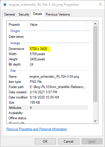
Once we’ve found an appropriate image we will want to make a note of the exact size. This can be found by right-clicking on the image file, selecting properties, and navigating to the details tab.
Resizing Flownex Canvas
The canvas in Flownex can be resized to match this resolution by right-clicking on the canvas, selecting edit page, and populating the correct inputs:

Applying Background Image
The background image can be applied by clicking the radio button next to Style in the Appearance subcategory. Here we will change the Fill Style type to Image, then click the Select Image button:

The images saved locally to this project will appear here. To add an image we simply click Add Image, navigate to the image of our choice, and click open. Now that it is available as an option we select the image in the Image Selector Gallery and click OK.

We can press OK in the Styles Editor to confirm our changes and we should now see our added image as the new background!
Bonus Tips!
- Adjusting the Fill Style opacity can fade out the background image so that it doesn’t overwhelm the Flownex components placed on top.
- Turning off the grid under the View ribbon can make the canvas a bit more aesthetically pleasing and makes it easier to read text on the background image.
