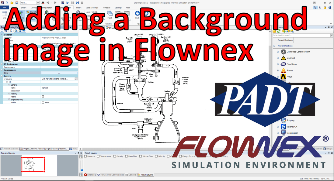
I’m going to attempt to write a recurring blog post on Fridays with tips and tricks in Flownex that I have discovered over the years. This post will be the first of many! If you enjoy please subscribe.
Flownex Tech Tip #1
In this post I will go over what is usually the first step in any network I build. Adding a background image not only helps me lay out my network but also helps colleagues and clients understand networks at a very quick glance. In this example I am using Flownex version 8.12.7.4334
Choosing an Appropriate Image
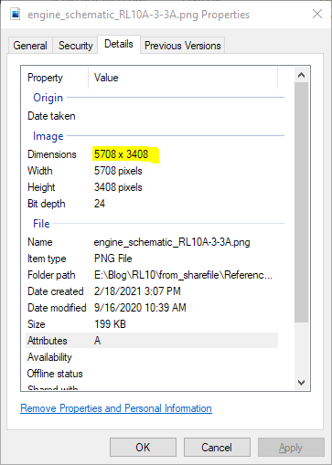
The first thing we want to do is to make sure that the image size is such that it’s reasonable in size both resolution-wise (so it doesn’t appear pixelated), and right-size so that components don’t appear too small when placed on top. I recommend something in the multi-thousands of pixels both in width an height. 3000 pixels at a minimum. I usually shoot for around 10,000 wide by 5,000 high if the background image will be landscape. For very complex, large networks, it may make sense to go much larger.
Once we’ve found an appropriate image we will want to make a note of the exact size. This can be found by right-clicking on the image file, selecting properties, and navigating to the details tab.
Confirming Image Resolution
Resizing Flownex Canvas
The canvas in Flownex can be resized to match this resolution by right-clicking on the canvas, selecting edit page, and populating the correct inputs:
Editing Canvas Inputs
Applying Background Image
The background image can be applied by clicking the radio button next to Style in the Appearance subcategory. Here we will change the Fill Style type to Image, then click the Select Image button:
Styles Editor
The images saved locally to this project will appear here. To add an image we simply click Add Image, navigate to the image of our choice, and click open. Now that it is available as an option we select the image in the Image Selector Gallery and click OK.
Image Selector Gallery
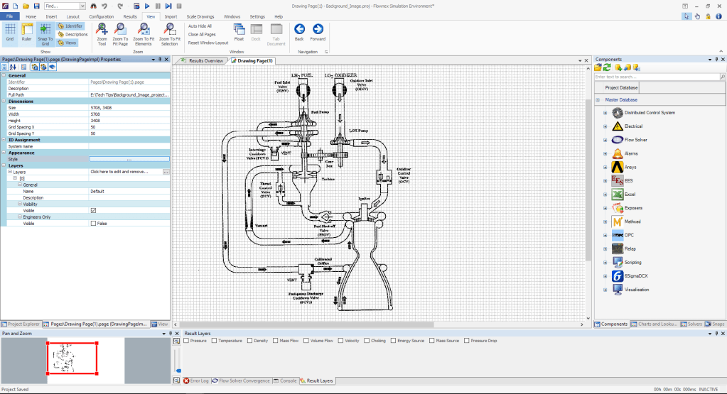
We can press OK in the Styles Editor to confirm our changes and we should now see our added image as the new background!
Drawing Canvas with Background Image
Bonus Tips!
Adjusting the Fill Style opacity can fade out the background image so that it doesn’t overwhelm the Flownex components placed on top.
Turning off the grid under the View ribbon can make the canvas a bit more aesthetically pleasing and makes it easier to read text on the background image.
When we engineers are building a new system or iterating on an existing design it can be expensive. Simulating a full system level model in a 3D CFD program can take days. Making iterative changes to an existing system can be costly or even impossible. Utilizing a one-dimensional system modeler like Flownex allows us to analyze many different designs very quickly, on the order of seconds or minutes.
Flownex is a thermal-fluid network modeler. It is a simulation tool that allows for 1D fluid modeling and 2D heat transfer. It uses a variety of flow components, nodes, and heat transfer elements to model the entire system we are interested in analyzing. It solves conservation of mass, momentum, and energy to obtain the mass flow, pressure, and temperature of fluids and solids throughout the complete network. Because of this approach we can analyze large, complex networks very quickly, iterate on designs, and even run short or long transient simulations with ease.
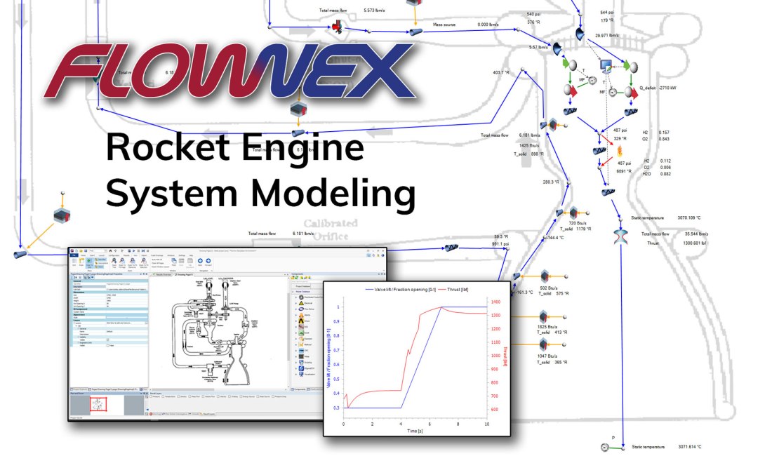
In the example today we are looking at a version of the RL-10 rocket engine, which has been a staple in the delivery of satellites into orbit and an essential part of many spacecraft. The specific iteration of the RL-10 we will be using for building our network model is the RL10A-3-3A. A good place to begin with any system model is a system schematic:
In Flownex we can assign an image (could be from a P&ID diagram, a CAD cross-section, or even a satellite image!) as the background for our drawing canvas. We simply need to right-click on the drawing canvas and select Edit Page to bring up the drawing canvas properties.
Clicking on the action button under Appearance > Style brings up the Styles Editor. Here we can change the fill style to Image and select the appropriate image for our background.
In the case of the RL-10 we can use the image from figure 2 as our background image. We may want to consider adjusting the opacity of the image so that it blends into the background a little bit more.
In Flownex building a system model is as simple as drag and drop. We can build our rocket engine using a variety of flow components from the Flow Solver library. To build the RL-10 system model we will be usingthe following components:
CEA Adiabatic Flame component to model combustion.
Composite Heat Transfer component to model thermal transport through pipe-walls to ambient and to model the regen.
Boundary Conditions to constrain our system at the inlets and outlet.
Basic Valves to model the different valves in the system,
Flow Resistances to model specified losses where appropriate.
Flow Interfaces to model the fluids entering the combustion chamber (to transfer fluid properties as we switch from two-phase O2 and H2 to gaseous fluids for modeling combustion.
Pipes for modeling various flow-paths.
Restrictors with Discharge Coefficient for our injection ports to the combustion chamber.
Restrictors with Loss Coefficient to model both the Calibrated Orifice and the Venturi contraction/expansion.
Basic Centrifugal Pumps for our Fuel and LOX pumps.
Simple Turbine to model the Fuel Turbine
Shafts to connect our different pumps mechanically.
Gearbox is used to connect the shafts between the LOX pump and the Fuel Pump.
Exit Thrust Nozzle to determine total thrust.
A Script is used in assigning O2 properties prior to combustion.
The components may be dragged and dropped from the component library onto the drawing canvas to build our system model. We can also copy and paste components that are already on the canvas into different locations. This can be especially useful when the same inputs for say, a pipe, are used consistently throughout the model. All components have both Inputs and a Results associated with them as seen in the figure below. This is how we will define our flow components.
The completed model of the RL-10 Rocket Engine can be seen below. There are a few simplifications; we are using composite heat transfer components to model free convection to a specified ambient temperature (as though this was a land-based test). Rather than tie the actual temperatures and flow conditions in the nozzle to the regen we are using assumed temperatures and convective heat transfer coefficients. For additional fidelity we could model the heat transfer between these two flow paths with calculated convective heat transfer coefficients and we could model cross-conduction along the pipes which deliver the fuel and oxidizer to the combustion chamber. With additional effort, more complex use cases could also be simulated.
For the sake of demonstration we set up a transient action to slowly vary the oxidizer control valve fraction open; starting at 30% and ending at 100% open and observer the change in thrust at the nozzle as a function of this changing transient action.
Plots may be easily added by dragging a Line Graph from the Visualization > Graphs section of the component library onto our canvas. To choose the characteristics we would like plotted against time we simply need to drag and drop the desired inputs or results onto our newly placed line graph.
RL-10 Transient Thrust Plot
We can plot both the oxidizer control valve fraction open and the thrust versus time to observe the thrust reaction to the opening of the valve. The thrust plot has some jumps that are likely due to numerical singularities – with additional work this could be improved.
As can be seen, setting up complex system models in Flownex is relatively simple with most operations being drag and drop. For ease of sharing models with colleagues or customers adding a background image makes it very easy to see how the flow components in the model correspond with a system schematic. Setting up and plotting the effects of operational transients is a breeze!
ANSYS Discovery is a wonderful tool for fast and first look structural, fluid flow, and thermal simulations. Discovery gives us the ability to modify geometry very quickly within the interface and to add or remove features to view realtime simulation reactions. This allows us to quickly iterate, explore design changes, and better understand interaction between our design and the environment. Today we are going to be investigating the pressure profile on the exterior of a travel trailer being pulled behind a truck down the highway.
Truck and Trailer with velocity streamlines
In this analysis we are using a 2018 Chevy Silverado 2500 model pulled from GrabCAD with a generic 25 foot travel trailer. Based on described experience we’ve noticed that the roof and sidewalls of a moderately sized travel trailer seem to bow outwards at highway speeds near the front of the trailer. The first thing to do is to put this model in an enclosure and prescribe a flow condition at the inlet and a pressure boundary at the outlet. Modeling the truck/trailer combo at a speed of ~55 mph (25 m/s) confirms that there is suction (negative pressure) present in these key areas:
Truck and Trailer in 25 m/s airflow, -500 Pa isosurface
While the actual roof and sidewall separating could be attributed to poor manufacturing processes we wonder if there could be a design change to minimize negative pressure/suction. One idea would be to incorporate some sort of turbulator to break up the laminar flow. I’ve seen turbulator tape in a zig-zag pattern used in aviation for this specific purpose so we’ll try recreating the travel trailer equivalent and see how it goes.
I started with a zig-zag pattern about 4″ tall on top of the trailer to see if I could “pop the bubble”
This did have the intended consequence and it was curious to see how much impact the turbulator on top of the trailer had on the negative pressure at the sidewall of the trailer:
The next thing I wanted to try was moving the turbulator forward or backward to see the effects. Moving the turbulator towards the aft of the vehicle has limited effects but moving it to different locations within the suction “bubble” seems to effect our -500 Pascal isosurface:
This would seem to indicate the presence of a “sweet spot” for turbulator location that merits further research in either the “Analyze” mode within Ansys Discovery or within Ansys Fluent.
Before I hang up my coat I’d like to investigate one alternate design that I’ve seen more often in automotive applications. I’m going to try adding vertical pillars and see how that goes:
We can easily change the height and position of the pillars to see the resultant effects on the pressure isosurface. The pillars also have a significant effect on the suction bubble but I notice that it has less effect on the suction on the sides of the trailer.
Using Discovery we can quickly and easily iterate on designs, get a first-view of the physics, and determine which change or design merits further investigation. In this analysis we can see that there is most definitely a suction profile at the front of a generic travel trailer. If the suction proves damaging we can see that there are several design changes which will help to mitigate this effect.
For more information on ANSYS Discovery please reach out to info@padtinc.com