Reading values from Excel component into Flownex Scripts!

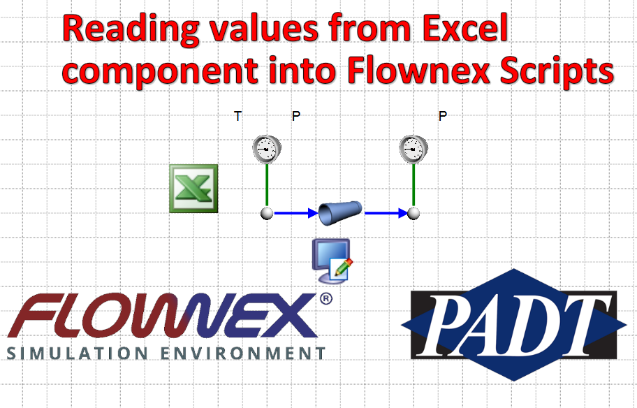
Today we’re going to explore how we can directly reference specific cells in Excel workbooks via script. By building the direct reference in the script we can avoid having to assign specific cells as outputs and we can also avoid having to use data transfer links which can clutter our work canvas.

Code Snippets

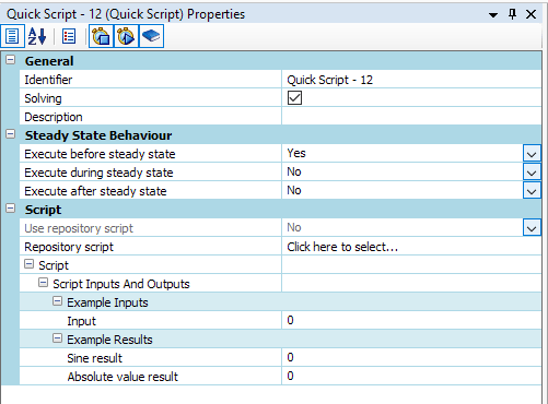
Depending on when we want the script to execute we should choose the appropriate function to make this part of. Since I want this to be called every cycle I will make this part of the “Execute” function.

//script main execution function - called every cycle
public override void Execute(double Time)
{
//new code to go here	
}

The first bit of code we’re going to use will link our script to the excel file “Workbook (2).xlsx” in the Flownex project directory.

SpreadsheetGear.IWorkbookSet workbookSet = SpreadsheetGear.Factory.GetWorkbookSet(); 

// Path to where Flownex Project is located
System.IO.DirectoryInfo projectpath = new System.IO.DirectoryInfo(Project.ProjectRootPath);	        
		
// Create Workbook object linked to .xlsx file or .csv
SpreadsheetGear.IWorkbook workbook = workbookSet.Workbooks.Open(projectpath + "\\Tasks\\ExcelWorkBooks\\Workbook (2).xlsx"); 

Now that we’ve created our workbook object connected to the Excel file we can read in values from cells in a couple of different ways.

To read from an explicit cell (A1),

// Read from Cell A1 in Sheet 1
double excel_value_1 = Convert.ToDouble(workbook.Worksheets["Sheet1"].Cells["A1"].Value); 

to read from a set row and column,

// Read from Row 4, Column 1 in Sheet 2 (Note: row and column indices start at 0)
double excel_value_2 = Convert.ToDouble(workbook.Worksheets["Sheet2"].Cells[3,0].Value); 

If the value in the Excel cell is a string we can use the following,

// Read text from Cell B1 in Sheet 1
string excel_value_3 = workbook.Worksheets["Sheet1"].Cells["B1"].Value as string; 

There we have it! These are now internal variables to the script. To assign them as output variables we can use the following syntax (this is all still within the Execute function).

//Save Value to Output Script Variable
Output1.Value = excel_value_1;
Output2.Value = excel_value_2;
Output3.Value = excel_value_3;

Then, as per the usual, we’ll need a bit of code to initialize these output variables and make them visible/usable outside of the script.

//constructer initializes parameters
	public Script()
	{
		_Output1 = new IPS.Properties.Double();
		_Output2 = new IPS.Properties.Double();
		_Output3 = new IPS.Properties.Text();
	}

	//property declarations to make
	//parameters visible to outside world
	[PropertyUsage(UseProperty.DYNAMIC)]
	public IPS.Properties.Double Output1
	{
		get
		{
			return _Output1;
		}
	}
	
	[PropertyUsage(UseProperty.DYNAMIC)]
	public IPS.Properties.Double Output2
	{
		get
		{
			return _Output2;
		}
	}
	
	[PropertyUsage(UseProperty.DYNAMIC)]
	public IPS.Properties.Text Output3
	{
		get
		{
			return _Output3;
		}
	}
}

Happy Friday and Happy Scripting!

Using a Table for Transient Actions in Flownex

Happy New Year! Today I want to show how we can easily use the new “Table” option to vary an input to our transient simulation. In this demo I am using Flownex version 8.12.8.4472.

Building the Fluid Network

If you’re most interested in how to implement the table for the transient inputs feel free to scroll past these next few sections. We’re going to go over the basic network building steps in case the information is found useful.

I chose to use a very simple network of a pipe with water flowing through it exposed to ambient air. We’ll use commercial steel for the pipe, with an inner diameter of 1 inch and a length of 100 feet. In my mind I’m pretending this is an irrigation line and as such I will add a restrictor at the end to represent something like a sprinkler head.

Heat Transfer to Ambient

The next thing we’ll want to do is model the heat transfer to ambient by way of a Composite Heat Transfer element. I have the upstream side connected to my pipe and will take advantage of that when getting areas for conduction and convection.

We can change the conduction areas drop-down to “use upstream pipe areas” and add an appropriate thickness and material type:

For upstream convection (water side), we can choose an appropriate correlation for calculating the convective heat transfer coefficient. Notice where we are obtaining inputs from the area specified in conduction and from the attached flow component. This saves us the effort of redundant calculations/inputs.

On the downstream side (air) we will set the composite heat transfer element for convection to ambient. For this set of inputs I still use the area specified in convection and then choose appropriate calculation operations for natural convection.

The key input we will be manipulating in the transient simulation is “T ambient” from the downstream composite heat transfer component. I will drag this property onto the canvas so we can easily monitor it during the run.

Setting up the Transient Scenario

What I’d like to model transiently is the effect of the changing ambient temperature on the temperature of the water in the pipe. To create a new transient scenario we go to the Configuration ribbon, click on actions setup, then in the Actions Setup Window we will right-click and “add scenario”

Since we will be manipulating the ambient temperature we will want to drag and drop this input into our newly created transient scenario as an action:

Using Table for Transient Action

We should choose “Table” under ValueType if we want to use the new Table option for varying our input transiently. I am going to use weather data for earlier this week for Phoenix, Arizona as my table of inputs. To make things easier I have converted the time to minutes after midnight.

TimeMinutes After MidnightTemp [°F]HumidityWindWind SpeedCondition
12:15 AM154283 %ESE6 mphFair
12:35 AM354186 %E5 mphFair
12:55 AM554086 %E5 mphFair
1:15 AM753889 %SE7 mphFair
1:35 AM953987 %SE9 mphFair
1:55 AM1154084 %ESE6 mphFair
2:15 AM1353985 %SE6 mphFair
2:35 AM1553887 %SSE7 mphFair
2:55 AM1753887 %SSE9 mphFair
3:15 AM1953887 %SE7 mphFair
3:35 AM2153886 %ESE7 mphFair
3:55 AM2353884 %ESE7 mphFair
4:15 AM2553886 %NE7 mphFair
4:35 AM2753885 %E8 mphFair
4:55 AM2953787 %E5 mphFair
5:50 AM3153781 %ESE8 mphFair
6:47 AM4073975 %ESE8 mphFair
7:50 AM4703781 %E6 mphFair
8:54 AM5344370 %ESE5 mphFair
9:50 AM5904854 %SE7 mphFair
10:50 AM6505250 %SW3 mphFair
11:50 AM7105544 %CALM0 mphFair
12:50 PM7705741 %WNW3 mphFair
1:50 PM8306136 %WNW5 mphFair
2:50 PM8906136 %CALM0 mphFair
3:50 PM9506332 %SW3 mphFair
4:50 PM10106332 %CALM0 mphFair
5:47 PM10675939 %S5 mphFair
6:47 PM11275544 %VAR5 mphFair
7:47 PM11875258 %SSE3 mphFair
8:47 PM12474871 %E5 mphFair
9:47 PM13074676 %ESE8 mphFair
10:50 PM13704581 %ESE6 mphFair
11:47 PM14274581 %ESE7 mphFair

The next step is to simply copy and paste or drag and drop our series of values into our new table.

Let’s run a transient and see how it behaves! Note that I’ve added an increment plot showing the temperature profile as a function of linear length of the pipe. I also modified my inlet boundary condition so that we’d have a more observable change in temp over the length of the pipe.

Although the outlet temperature stays relatively constant, if we look at the change overlaid with the changing ambient temperature we see the expected correlation. An interesting next step might be to incorporate the wind speed data and model the external convection as forced convection where we vary the wind speed according to our table.

Creating a Human Machine Interface in Flownex

Flownex Tech Tips!

No, robots are not taking over… yet… Luckily, Flownex has human machine interface controls available so that we can interact with our system simulation. Let’s go over how to maintain human control of our system using an HMI. For this demo I am using Flownex version 8.12.8

Visualization Library

In the Components pane near the bottom we can find our human machine interface (HMI) components in the Controls category. We have a few components here which we’ll go over use cases for. As a reminder, if we want to learn more about a specific component we can always select the component and press F1 on our keyboard to bring up the library manual for that specific component.

Dial

No, the phone call is not coming from inside the house! We can use the dial component to visualize any property, usually a result, in a dial interface. To use the dial component we simply drop it into our network and then drag and drop the property we’re interested in onto the component itself.

We must set the minimum and maximum values for our dial, in this case since we are reporting the pressure we will want the variable type to be Double. If we want to get fancy we can change our start degrees, amount of rotation, even replace the gradient background with an image from an actual dial!

IO Box

The IO Box is probably something we’ve already been using without even realizing it. This is what is created whenever we drag an input or result property onto the canvas. In the image with the dial we use an IO box to report the pressure in our reservoir. We can attach properties to IO boxes by dragging and dropping. In the properties of the IO box we can change the font, size, units, how many significant figures are reported, and more.

Progress Bar

The Progress Bar is used in very similar situations as the dial however I find it to be particulary useful when reporting fill levels in containers or reporting valve fractions open. We’ll tie the “fraction open” of the restrictor component downstream of the reservoir to our progress bar.

Push Button

The Push Button can be used for a variety of operations (selectable via drop-down in the inputs). I most often use these to run scripts, start, or stop a transient simulation. We have all of the similar formatting options as we’ve seen with these other tools. It is important to note that in order to interact with the push button we need to be in “Interact Mode” found on the home ribbon.

Toggle Button

The Toggle Button is going to be similar to the push button but has distinctive on vs off characteristics. We most often would use this to set a property. This can, again, be set up by dragging and dropping the property onto the button. What I’ll do in this example is have the toggle button set up to toggle our downstream pressure boundary condition between 14.7 psi and 50 psi to simulate an overpressure event. We can go into the different style menus to make our button more aesthetically pleasing and change the text, etc.

Track Bar

The Track Bar is a slider which allows us to vary an input via interaction. We’ll use two track bars in this example; One to control the mass flowrate at the inlet and a second to control the fraction open of the restrictor. To tie a property to a trackbar we again drag and drop the property and then update the track bar’s minimum and maximum values to give us the range of operation. The complete network with all of the HMI components can be seen below (remember we are in “Interact” mode):

Avoid Spiderwebs with Direct References in Scripts

Flownex Friday Tech Tips!

It’s officially Spooky Season! In between episodes of Squid Game and re-watching Hubie Halloween I thought I could make things a little less scary by demonstrating how to get rid of the spiderwebs in our projects (AKA Data Transfer Links). We use these often with scripts, which can be very powerful, but as our networks get more complex we may want to avoid the clutter/attracting spiders.

Quick Script vs Full Script

If we’re not scared of a little C# we may decide to start with a full script. I, personally, like to use a quick script so that I can use the table inputs to define my script inputs and results.

Calling a Specific Component

We will identify the component we want to read/write to by the unique Identifier. This can be found in the input properties for the component. In this example we’ll use a pipe component. By default this would typically be “Pipe – 0” or “Pipe” followed by some other integer. This field is editable so you can change it, but it must remain unique to that specific component.

We can either specify the identifier as a string explicitly in the script:

//Referencing component "Pipe - 0"
IPS.Core.Component Pipe = Project.GetComponent("Pipe - 0");

Or we can have this as an text-type input to the script so that we can change the reference more easily. In this example we have a text variable “ComponentIdentifier”:

//Referencing component which is defined by input "ComponentIdentifier"
IPS.Core.Component Pipe = Project.GetComponent(ComponentIdentifier.ToString());

Note that we are using the ToString function to convert our text variable to a string.

Reading from Component

Now that we have our Pipe component referenced in the script we can read any of the results into our script via their display identifier using the following syntax:

//Reading from flow component
IPS.Properties.Double T_1 = Pipe.GetPropertyFromFullDisplayName("{Flow Element Results,Generic}Total temperature
") as IPS.Properties.Double;
Pipe_Temp.Value = T_1;

Note that we must use a internal variable. in this case “T_1”, to read the temperature before we assign that to the value of our script result “Pipe_Temp”.

A quick trick to determine the display name is to right-click on the result you’re interested in and select “Copy display identifiers to clipboard”.

Writing to Component

The process of modifying a component input with values from the script is very similar. We can use the above trick on our Inputs for the component to find the display identifier for the pipe diameter in this example.

//Write to component
IPS.Properties.Double diameter = Pipe.GetPropertyFromFullDisplayName("{Geometry,Inlet}Diameter") as IPS.Properties.Double;
diameter.Value = Pipe_Diameter;

Summary

Here is how we’ve set up the quick script, as you can see it is really not that scary:

And the snippet of code from the quick script:

//Identify Component
IPS.Core.Component Pipe = Project.GetComponent(ComponentIdentifier.ToString()); 

//Read from component
IPS.Properties.Double T_1 = Pipe.GetPropertyFromFullDisplayName("{Flow Element Results,Generic}Total temperature") as IPS.Properties.Double;
Pipe_Temp.Value = T_1;

//Write to component
IPS.Properties.Double diameter = Pipe.GetPropertyFromFullDisplayName("{Geometry,Inlet}Diameter") as IPS.Properties.Double;
diameter.Value = Pipe_Diameter;

Happy Friday and Happy Coding!

Modeling a Fire Suppression System in Flownex

Flownex Friday Tech Tips!

Today I’m going to go through my workflow of modeling a fire suppression system in Flownex. This particular system is designed with an aircraft in mind. We’ll go over typical workflow and transient setup using Flownex version 8.12.8.4472

Background Image

See my post on adding a background image for in-depth step-by-step direction. I first set up a background image so I have an easily understood flow schematic to reference in my Flownex build. This also is particularly useful when showing or passing the network off to a colleague or customer who may not have intimate familiarity with Flownex. The image I used in this demo is from this paper by Jaesoo Lee.

Choosing the Appropriate Flow Components

In this model I’ve got a storage bottle, a distribution pipe, and some injection nozzles. I know that I want this to be able to handle two-phase and I know I am pressurizing the bottle with N2 so I will use the Container Interface components to represent the bottle. I will use pipe components for the distribution line, and for the nozzles I will simply use restrictors with discharge coefficients.

Container Interface – Top

Container Interface – Bottom

Pipe

Restrictor with Discharge Coefficient

Building network of components and entering geometry

While building this network I realized I was missing one additional component. I needed to add a valve to open the bottle and release the fire suppressant (HFC-125) and a valve representing a vent to the top portion of the tank which we will leave fully closed.

We need to specify our initial pressures, mass fractions, and a temperature on the storage bottle. We also need an outlet pressure and temperature to fully constrain our model. I use a “view” node on my nozzle so that I only need to specify a single outlet boundary condition.

Transient setup

For this transient analysis I am going to open the valve and see how quickly the suppressant discharges from the system. The first thing we will want to do is to remove any boundary conditions that we want to be “free” during the transient. I’ll remove all of the boundary conditions at the storage bottle so that Flownex will calculate the remaining pressure as our system discharges.

I also need to specify our timestep and simulation length. We can do this under the Scheduler properties which can be found in the Solvers pane on the right side of the GUI. I chose a timestep size of 20ms and a total simulation duration of 2 seconds.

Solve Steady State, Snap and Run!

To get a stable transient simulation it’s best to start from a converged steady state. At this point I’ll solve steady state, addressing any warnings that arise. Then we will want to save a Snap of the solve (so that we can load the snap to get back to initial conditions for any future transient runs).

At this point we should be good to run our transient analysis! I’ve added a plot of the pressure in the bottle and pressure just before the nozzles vs time to this project as well:

Scale Drawings in Flownex

Flownex Friday Tech Tips #17

Flownex has a pretty neat utility to capture geometry from a scale drawing and apply those inputs automatically to your flow network. In todays tip we’ll go over a simple example of how to implement this. We are using Flownex Version 8.12.8.4472

Adding a Scale Image

To apply a scaled image in our Flownex network we will want to navigate to the Scaled Drawings ribbon. Here we can click on Generate Scale Drawing and import our desired image. For this demo I’m using a waterblock idea I sketched up a long time ago to try to fix the overheating issue I was having with my Xbox 360.

Applying Dimensions to Network Components

We’ll notice that some dimensions are automatically associated with our new drawing. For instance, if we put some pipe components in to represent the flow paths we can see that the lengths are automatically updated. I know that these finned sections were about 90mm long so this checks out with what the scaled drawing is using.

We also have the option of associating dimensions with line segments we draw on the canvas. Since the cross-section of this flow path is rectangular perhaps a “duct” component would be better suited so that we can capitalize on the geometry association:

Other Useful Scale Tools

There are a few useful measurements we can do using the scale drawings utility that I didn’t highlight in this demo. Point measurements and Link Points can be extremely useful in a variety of scenarios; A couple of examples might be to define connection points on rotor cavities or elevations of connections to some type of container.

Bonus Tip!

  • If your CAD is evolving we can swap out that image and then updating the measurements in our flow network is as simple as moving the components back into their correct places; Inputs update automatically!

Simple Scripting in Flownex

Friday Flownex Tech Tips #15

Scripts can be very powerful additions to our network building toolbox. But we don’t need to have a degree in computer science to use them! The quick script makes integrating scripts into our network quite simple. In this tip we’ll go over how to set up a quick script in Flownex version 8.12.7.4334

Example Problem

In this demo I’m going to model a small pipe that is horizontal and perpendicular to the flow of a much large duct. We’re going to use a script to utilize our own correlation for determining the convection heat transfer.

What I’d like to accomplish is to apply the Churchill-Bernstein correlation for cylinder in a cross-flow to calculated the Nusselt number and in turn the convection coefficient.

Example Network

To build this network I’m just going to use a couple of pipe components and a composite heat transfer component. I’m assuming the cross-sectional area of the larger duct is not so impacted by the presence of the cross-pipe that we need to calculate any losses associated with it.

Quick Script

Quick scripts are located in the components pane near the bottom. To add a quick script we’ll simply drag and drop the script onto the canvas. Notice the inputs available for the quick script, we get to choose when it executes, and then we’ll notice that there are some example inputs and results. Since this script is going to be used to apply a correlation during the solve we’ll want this script to execute during steady state.

To edit the script we’ll need to double click on the quick script component. Then we’ll need to define our inputs and results. In this case we’ve got quite a few inputs and results to define.

The most challenging part, in my opinion, is simply getting the correct syntax for C#. Luckily there are a myriad of resources online for C# syntax which makes things a bit easier. In the below image I’ve added the mathematical operations to calculate Re_D and Nu_D using the Churchill and Bernstein correlation.

Connecting Script to Components

We’ll connect the script to our components using data transfer links. We’ll need to populate our script inputs with results from our network and then update the heat transfer input using the results from our script.

Once we’ve connected all of the data transfer links with the appropriate properties we ought to be able to solve!

Real-Time Plotting in Flownex

Flownex Tech Tip #14

Today’s tech tip will be short and sweet. We’re going to go over how to do a real-time plot in Flownex. In this example we’re using Flownex version 8.12.7.4334

Adding a Time Dependent Graph

For a time dependent graph we will choose the Line Graph under the Visualization library on the Components pane. We can drag and drop the variables we’d like to see plotted here. I’m going to look at the pump speed (rpm), the valve fraction open, and the mass flow through our network.

On the graph properties we’ll likely want multiple Y-axis enabled so that the changes are easily seen as a function of time.

Real-Time Transient

To have our transient analysis solve in real-time we will need to go to the Solver Ribbon and click on Scheduler to access our transient settings. Here we can change the Running Speed to “Realtime”

Now when we run our analysis we will get real-time response! This comes in super handy when building human machine interfaces in Flownex for testing operations, when we want to observe response of controls systems, or observing start-up/shut-down type scenarios.

Lucky Number 13! Parameter Sheet Tricks!

Flownex Tech Tip #13

It’s Friday and time for the 13th Tech tip! Today we are going to go over some simple parameter sheet tricks and best practices. Parameter sheets are incredibly useful for running many different design or operation analyses. Let’s go over how best to utilize their functionality. In this example we’re working in Flownex version 8.12.7.4334

Parameter Sheet Setup

Probably the most critical thing to know when working with Parameter Sheets in Flownex is to make our edits through the setup interface. This is where we define the connection between Flownex and the worksheet.

As we recall, adding either inputs or results to our parameter sheet is as simple as dragging and dropping them into the different columns.

Renaming Parameter Columns

We may find that we’d like a more descriptive name of an input or result parameter than simply
“Pressure” or “Temperature”. We can rename the columns and this must be done via the parameter table setup. If we were to change the name in the worksheet it will be overwritten by the setup when the model is solved.

Rearranging Parameters

We may decide after creating a parameter table that we need to go back in and add a new column between existing input or result parameters. This should be done, again, through the setup. We will add our new parameter to the first open column and then move it within the setup.

*Important Note: Cell references in Excel are explicit in parameter sheets. If we are performing calculations in the parameter sheet using cell references and we rearrange columns these formulas will need to be updated.

Bonus Tip!

Sizing Pumps and Manually Specifying a Pump Curve in Flownex

Flownex Tech Tip #12

As a System Engineer you may not always already have equipment decided on for your particular network. Flownex makes it easy to start from scratch and will help determine the equipment necessary to meet the flow or process requirements. In today’s tip we’ll go over how to size a pump using the basic centrifugal pump component and how to manually enter pump curve data. We are using Flownex version 8.12.7.4334

Sizing a Pump

In our example scenario let us pretend we are sizing a pump for a cooling water circuit. We are tasked with finding a pump which will deliver water at a rate of 1 kg/s to the heat exchanger. We know our upstream and downstream boundary conditions as well as the heat added at the exchanger and the speed at which we will be operating the pump.

Choose the appropriate flow component

There are a few different pumps available in Flownex:

Basic Centrifugal Pump: Used when we do not have a pump chart available, particularly useful when sizing a pump.

Fan or Pump: Used when a pump chart is available for modeling either compressible or incompressible flows.

Positive Displacement Pump: Used for modeling rotary and reciprocating pumps where the fluid is incompressible, non-Newtonian, or a slurry.

Variable Speed Pump: Similar to the Fan or Pump but with the ability to interpolate between fan/pump curves for different speeds of rotation.

In this case we’d choose the Basic Centrifugal Pump. This is found in the component pane under Turbos and Pumps. Since we only know the RPM we can enter it in the inputs under Speed at BEP:

Recall we don’t know what the design of the pump will be. Since all we know is that the mass flow rate needs to be 1 kg/s we will check the box for fixed mass flow and then select to change design to target our desired flowrate.

Once we hit solve our pump design inputs will be populated such that our desired mass flow rate is achieved. We can cross-reference these values with available pumps to choose the appropriate component for our network!

Specifying a Pump Curve

If we already know which pump we are using, or perhaps are trying to decide between several available pumps, we may need to add these pump curves to Flownex. To add a pump curve we will navigate to the Charts and Lookup Tables pane > Project Database > Flow Solver > Turbos and Pumps. In this scenario we are looking at a single speed pump so we will right-click on Pump and Fan Charts and Add a Category.

We can name our category whatever is appropriate and then right-click on the newly created category to add our own pump chart.

To edit the newly created pump chart we can either double-click on it or right-click and select edit. Now we simply specify the Reference Density and then fill out the table with the relevant data points. To speed things along we can copy and paste a table of data points from excel or whatever source we get this curve from. Don’t forget to check your units!

Bonus Tip!